This dissertation is submitted for the degree of Doctor of Philosophy at the University of Cambridge, and is an account of work carried out in the Department of Materials Science and Metallurgy from October 2002–2005 under the supervision of Professor H. K. D. H. Bhadeshia. This work is to the best of my knowledge original, except where acknowledgement and reference is made to previous work. Neither this, or any substantially similar dissertation has been or is being submitted for any degree, diploma or other qualification at this, or any other university. This dissertation contains less than sixty thousand words.
Parts of this thesis have been published previously in journals, much of Chapter 5 has been published in “Three-Dimensional Atom Probe Analysis of Carbon Distribution in Low-Temperature Bainite” by Peet, Babu, Miller and Bhadeshia [1]. Chapter 6 presents results from two alloys, the results of one have been presented in “Tempering of a Hard Mixture of Bainitic Ferrite and Austenite” by Garcia–Mateo, Peet, Caballero and Bhadeshia [2].
I gratefully acknowledge the Engineering and Physical Sciences Research Council, Corus Plc (now Tata Steel Europe Ltd), the Isaac Newton Trust for funding my study and the Worshipful Company of Iron Mongers and the Shared Research Equipment (SHaRE) User Facility at Oak Ridge, which enabled me undertake atom probe studies presented in this thesis. I am grateful to Prof. D. J. Frey and Prof. A. L. Greer for the provision of laboratory facilities in the Department of Materials Science and Metallurgy.
Many thanks to all the friends and colleagues in the phase transformations and complex properties group for their friendship. Special thanks to Miguel Angel Yescas-Gonzalez, Shingo Yamasaki, Kazukuni Hase, Teruhisa Okumara, Mohamed Sherif, Saurabh Kundu, Carlos Garcia–Mateo, Thomas Sourmail, and Rose Yan for their useful advice and discussion which aided the work presented here.
It gives me pleasure to thank Mary Vickers, David Vowles and David Nicol who provided much useful assistance and advice for X–ray diffraction, scanning electron microscopy and transmission electron microscopy, and Harald Dobberstein and Jon Rickard in the Cavendish Laboratory for their assistance in the use of the focused ion beam microscope. Without Mike Miller, Kay Russel and Suresh Babu the atom probe work would not have been possible. I would also like to thank Marimuthu Murugananth for his friendship and assistance during my visit to Oak Ridge. Thanks to Kevin Roberts and to Brian Whitemore for their assistance with various experiments.
I also would like to thank all who have contributed to open software used to prepare this thesis, especially the developers of the Linux kernel, gcc, g77, gfortran, Debian, Redhat, Gnome, vi, Gnuplot, xfig, Gimp, inkscape and LATEX.
I am greatly indebted to Prof. Harshad Kumar Dharamshi Hansraj Bhadeshia for his guidance, advice, enthusiasm and patience.
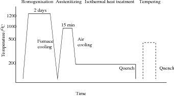
This thesis concerns a special class of novel bainitic steels, which can transform to bainite at around 200∘C. The microstructure has been labelled ‘super–bainite’, a mixture of fine bainite plates (20-40 nm thickness) in a matrix of austenite which is highly enriched in carbon. These high strength steels have found application as armour plate, and there has been further research to utilise them for aerospace applications.
The introductory chapter of the thesis contains a literature survey, starting from general background describing the solid–state transformations, and then developing with particular reference to earlier work on bainite, carbide–free bainitic steels, and on this new class of low–temperature bainitic steels.
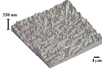
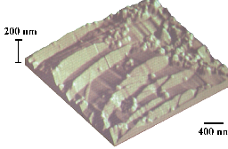
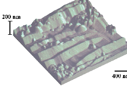
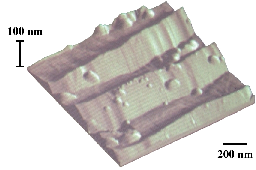
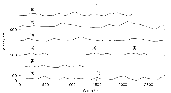
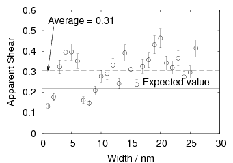
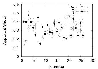
Bainite transforms by a displacive mechanism, and chapter 2 characterises the surface relief due to transformation using a high–resolution surface technique. The measured shear component is larger than expected from past experience. This large shear component is consistent with the slender aspect of the ferrite plates. It may be that the small size of the features makes it much more difficult to measure the shear component as compared to transformation at higher temperatures.
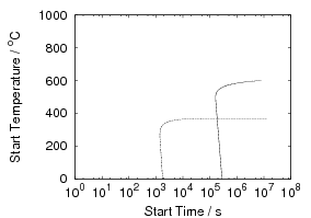
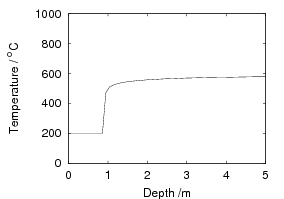
Since the strengthening mechanism is a result of transformation, these steels offer a unique opportunity to achieve high strengths in large section sizes. In chapter 3 results of transformation of large samples are reported and experimental results are compared against calculated continuous cooling curves. It is demonstrated that uniform transformation of bulk sections is possible, and methods are presented that can be used to estimate limiting section sizes from the calculated time–temperature–transformation curves. It was found that in the alloy studied, the isothermal transformation kinetics were faster than calculated. It is proposed that this may be due to the formation of pro–eutectoid cementite.
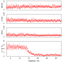
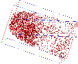
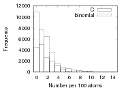
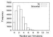
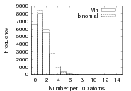
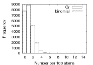
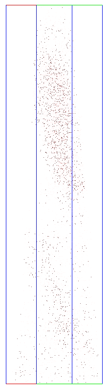
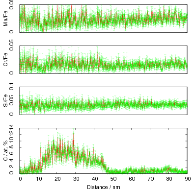
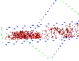
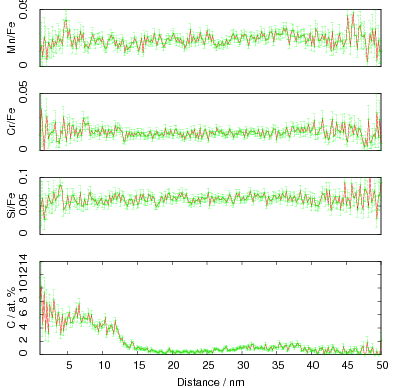
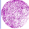
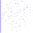
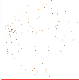
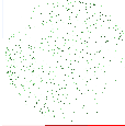
The microstructure due to transformation at 150 and 200∘C was characterised by X–ray diffraction, hardness testing, and thin–foil electron microscopy as presented in chapter 4. The bainite plates size was determined to be 39±1 nm after transformation at 200∘C but unexpectedly increased upon transformation at 150∘C. As previously reported, significant carbon supersaturation occurred in the austenite by transformation at 200∘C as limited by free–energy change to super–saturated bainite, however no enrichment could be measured in the austenite transformed at 150∘C. This indicates that there is a optimum temperature for achieving both fine plate size, and stabilisation of retained austenite. The microstructure as a result of transformation at 200∘C was characterised by atom probe tomography (chapter 5). These direct measurements of carbon content are in agreement with the X–ray diffraction data reported in chapter 4. It can also be confirmed that substitutional element partitioning does not occur from the bainitic ferrite during transformation. The results are fully consistent with the displacive nature of the transformation.
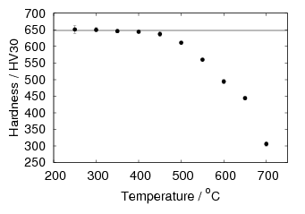
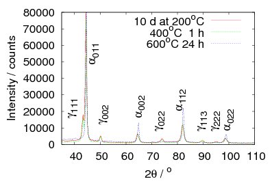
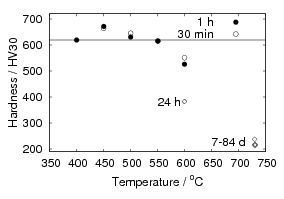
The final two chapters of results deal with tempering of low–temperature bainite. The loss of hardness is consistent with the major strengthening mechanism being due to the plate size. X–ray measurements show that carbon in ferrite slowly reduces with increasing temperature, along with the recovery of heterogeneous strains. In contrast, hardness drops more rapidly after some critical temperature is reached. Carbides were identified by both X–ray diffraction of extracted residues, and using atom probe tomography, to be cementite. Tempering for 30 min at 400 and 500∘C resulted in a fine carbide size around 10 nm, which can also contribute to strengthening, as well as being ideally positioned to prevent coarsening of the ferrite. Austenite decomposition takes some time, and a small amount can be retained even at 500∘C for 15 minutes, or at 450∘C for 1 h.
The final chapter deals with general conclusions and proposes future directions of research based on the results. Further work is needed to fully characterise the tempering behaviour of these steels, particularly at lower tempering temperatures which may be relevant in some applications.
Novel high–carbon high–silicon steels have been developed by Caballero et al. [3]. The alloying of these steels allows a bainitic microstructure to form at unconventionally low temperatures. The resultant fine bainitic ferrite plates contribute significantly to the hardness and strength [3, 4].
Refinement of microstructure by transformation is an extremely attractive strengthening mechanism, introducing obstacles to dislocation movement, but unlike other strengthening mechanisms, not necessarily leading to a reduction in toughness [5]. Using transformation rather than deformation to introduce defects means that even large sections can be hardened.
These steels are a development of silicon–containing carbide–free bainitic steels. Silicon additions are known to prevent the formation of embrittling carbides during the bainite transformation [6, 7]. This results in a microstructure of plates of bainitic ferrite in a matrix of carbon enriched retained austenite1 . One advantage is the suppression of coarse carbides which can limit the toughness. The retention of austenite can also have a profound effect on the mechanical properties.
Alloying with silicon is also known to decrease the rate at which martensitic steels temper [8, 9]. Bainitic steels are more resistant to tempering than martensitic steels, because their strength is not predominantly due to supersaturation of carbon [10, 11]. Previous work on the high–carbon high–silicon steels shows that the microstructure can retain much of its high hardness upon tempering [3].
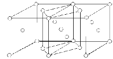
The susceptibility of iron to solid–state transformations between the two crystal structures which are stable at atmospheric pressure enables a huge variety of microstructures and mechanical properties to be generated in iron–based alloys by thermal treatments. These two structures are face–centred cubic (FCC) austenite and body–centred cubic (BCC) ferrite as illustrated in figure 1.1.
In pure iron the transition from ferrite to austenite and back to ferrite upon cooling and heating, is significantly influenced by magnetism. The energy difference between the two states is very small, and so alloying elements can have a large effect on the transition. Due to the industrial significance and scientific interest, many thermodynamic assessments have been made of iron–based systems so it is possible to model these effects by computation [12, 13].
Austenite is the stable form between 910 and 1390∘C in pure iron at atmospheric pressure. The face–centred cubic structure of austenite offers an optimum stacking in space for spheres, as first observed by Kepler [14] and recently proven by Hales [15]. Transformation from austenite to body–centred cubic ferrite is therefore inevitably accompanied by an increase in volume. Alloying elements can either substitute for an atom in the crystal lattice, or when the solute atoms are small enough they may occupy the interstitial sites between the larger solvent atoms. Carbon and nitrogen are relatively small and occupy interstitial sites in austenite and ferrite. Despite the greater packing efficiency the interstices in austenite are larger, resulting in higher solubilities. The volume increase when austenite transforms to ferrite is typically between 1 and 3% dependent on temperature, there are also significant differences in the solubility (table 1.1) and mobility of interstitial elements in austenite and ferrite. The diffusion coefficient at 910∘C being 1.5×10⁻⁷ cm2s−1 in austenite and 1.8×10⁻⁶ cm2s-1 in ferrite [16].
| Temperature /∘C | Solubility /wt% | Solubility /at.% | |
| C in γ–iron | 1150 | 2.04 | 8.8 |
| 723 | 0.80 | 3.6 | |
| C in α–iron | 723 | 0.02 | 0.095 |
| 20 | < 0.00005 | < 0.00012 | |
| N in γ–iron | 650 | 2.8 | 10.3 |
| 590 | 2.35 | 8.75 | |
| N in α–iron | 590 | 0.10 | 0.40 |
| 20 | < 0.0001 | < 0.0004 | |
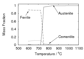
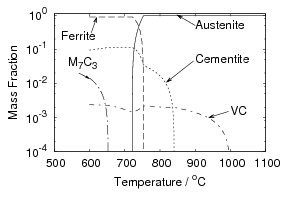
Iron and carbon also form an intermediate iron–carbide compound named cementite at equilibrium which has the stoichiometric formula Fe3C. The iron / iron–carbide equilibrium phase diagram, figure 1.2, represents the domains of stable phases as a function of temperature and composition assuming that graphite is suppressed.
All the solid state transformations from austenite to ferrite take place by nucleation and growth, with the parent and product phases coexisting separated by an interface. The formation of equilibrium phases is often preceded by that of a metastable phase which is quicker to form, due to a smaller activation energy for nucleation.
Bhadeshia [18, 19] proposed a classification considering all the transformations that occur in steels, which is consistent with all available experimental data, as summarised by the flow chart, figure 1.3. The different forms of ferrite are classified into those which grow by a displacive and those that grow by reconstructive mechanisms, as proposed by Guy [20]. The austenite decomposition reactions lead to Widmanstätten ferrite (αw), lower bainite (αlb), upper bainite (αub), acicular ferrite (αa) and martensite (α′) occur by a displacive mechanism, characterised by an invariant–plane strain resulting in surface relief and a plate or lath shaped transformation product. Reconstructive transformations include allotriomorphic ferrite (α), idiomorphic ferrite (αi), and pearlite (P). Since all the elements must diffuse during reconstructive transformation in order to achieve the structural change, these reconstructive transformations are not associated with shear strains. In the eutectoid decomposition reaction which leads to a pearlitic microstructure, ferrite and carbide phases grow ‘cooperatively’ with a common transformation front with the austenite.
Table 1.2 lists the key characteristics of phase transformations in steels after Bhadeshia [18, 21]. Consistency of a characteristic with the transformation concerned is indicated by √, inconsistency by ×, cases where the characteristic is sometimes consistent with the transformation are indicated by ⊗. Many of the characteristics presented in the table are discussed in the next section in the context of the bainite transformation.
The ability of the elements to re–arrange themselves into the a new structure plays an important role in both the nucleation and growth of the product phase. As can be seen in table 1.2, many of the transformation products necessitate diffusion and hence the critical role of temperature in determining structure.
Characteristic | α’ | αlb | αub | αa | αw | α | αi | P |
Nucleation and growth reaction | √ | √ | √ | √ | √ | √ | √ | √ |
Plate Shaped | √ | √ | √ | √ | √ | × | × | × |
IPS shape change with large shear | √ | √ | √ | √ | √ | × | × | × |
Diffusionless nucleation | √ | × | × | × | × | × | × | × |
Only carbon diffuses during nucleation | × | √ | √ | √ | √ | × | × | × |
Reconstructive diffusion during nucleation | × | × | × | × | × | √ | √ | √ |
Often nucleates intragranularly on defects | √ | × | × | √ | × | × | √ | × |
Diffusionless growth | √ | √ | √ | √ | × | × | × | × |
Reconstructive diffusion during growth | × | × | × | × | × | √ | √ | √ |
Atomic correspondence during growth; |
|
|
|
|
|
|
|
|
- shared by all atoms | √ | √ | √ | √ | × | × | × | × |
- for atoms in substitutional sites | √ | √ | √ | √ | √ | × | × | × |
During growth; |
|
|
|
|
|
|
|
|
- bulk redistribution of substitutional atoms | × | × | × | × | × | ⊗ | ⊗ | ⊗ |
- local equilibrium at interface | × | × | × | × | × | ⊗ | ⊗ | ⊗ |
- local paraequilibrium at interface | × | × | × | × | √ | ⊗ | ⊗ | × |
Diffusion of carbon during transformation | × | × | × | × | √ | √ | √ | √ |
Carbon diffusion-controlled growth | × | × | × | × | √ | ⊗ | ⊗ | ⊗ |
Co-operative growth of with cementite | × | × | × | × | × | × | × | √ |
High dislocation density | √ | √ | √ | √ | ⊗ | × | × | × |
Incomplete reaction phenomenon | × | √ | √ | √ | × | × | × | × |
Necessarily has a glissile interface | √ | √ | √ | √ | √ | × | × | × |
Orientation relationship within Bain region | √ | √ | √ | √ | √ | × | × | × |
Grows across austenite grain boundaries | × | × | × | × | × | √ | √ | √ |
High interface velocity at low temperatures | √ | √ | √ | √ | √ | × | × | × |
Displacive transformation mechanism | √ | √ | √ | √ | √ | × | × | × |
Reconstructive transformation mechanism | × | × | × | × | × | √ | √ | √ |
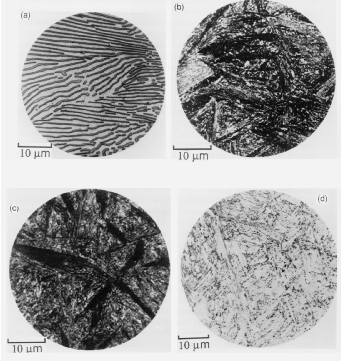
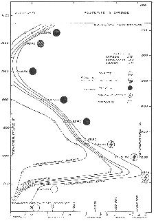
The bainitic microstructure was first identified as a result of systematic isothermal transformation experiments by Davenport and Bain [22], who reported the discovery of an ‘acicular, dark etching aggregate’ formed after isothermal holding between the temperatures for pearlite and martensite formation. The microstructures (reproduced in figure 1.4) were unlike martensite or pearlite observed in the same steel, and were found to be represented by their own ‘C–curve’ on the time–temperature–transformation (TTT) diagrams which they introduced as a convenient way to represent the time dependence of transformation at different temperatures. They suggested that the new microstructure ‘forms much in the manner of martensite but is subsequently more and less tempered and succeeds in precipitating carbon’. Figure 1.5 shows an example TTT diagram reported by Davenport and Bain for a high carbon alloy.
Describing the bainitic structure Hultgren also proposed that ‘needles of troostite’ (later named bainite) first formed as martensite needles which were then self–tempered [24] being able to reject carbon and form carbides due to the higher temperature of transformation than that associated with martensite.
An acicular or plate shape is often the result of a displacive transformation, as will be discussed later in this chapter. An explanation was therefore sought to explain the sluggish transformation of bainite in comparison to martensite. The martensite transformation is usually so rapid that it can often be regarded as only being dependent on temperature. At the time many wrongly supposed that martensite springs fully formed from the matrix rather than by a nucleation and growth mechanism [25]. It was argued that the slower growth meant that bainite must not be a martensitic transformation. Robertson made a study of the transformation rate of the microstructures formed upon quenching from austenite and proposed that the slow growth of the ferritic constituent of bainite is best explained by transformation being controlled by carbon diffusion [26]. Other work emphasised the similarity to martensite, and it was understood that bainite formed with a supersaturation of carbon [27, 28, 29, 30]. Vilella [31] and Bain [32] proposed that transformation involved the formation of flat plates which form abruptly, before decarburising at a rate depending on the temperature. The process to reject carbon from the ‘quasi–martensite’ was proposed to take millionths of a second.
It was recognised that the form of bainite was different in different temperature ranges as can be seen in figure 1.4. Mehl introduced the two main classifications of upper bainite and lower bainite [33], with lower bainite transforming at lower temperatures than upper bainite. Upper bainite has also been referred to as feathery bainite [25]. Intermediate forms were also recognised to exist as a result of continuous cooling transformations. Figures 1.4(b) and (c) show upper and lower bainite respectively. In the optical microscope lower bainite can be described as being similar in appearance to tempered high carbon martensites, while upper bainite more closely resembles low carbon martensite [34]. Observation by transmission electron microscopy later clearly demonstrated that the different types are due to the nature of carbide precipitation, and can be influenced by changing carbon content and temperature. In upper bainite, carbides precipitate from austenite between the plates which have become enriched in carbon, with the upper bainitic ferrite remaining free from carbides. In lower bainite there is also a finer dispersion of plate–like carbides inside the ferrite plates. Carbides have been observed to precipitate in a single crystallographic variant within a given ferrite plate, whereas in martensite tempering generally leads to precipitation of many variants [21].
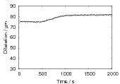
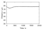
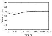
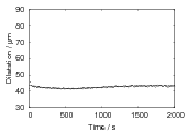
In steels where transformation to pearlite could be delayed, it could be observed that the maximum degree of transformation to bainite decreased with increasing temperature [35, 36] and there was a critical temperature above which bainite would no longer form. The transformation to bainite below this temperature would often stop, to be followed by pearlite [36]. Dilatometric experiments on a range or steels of different carbon contents, showed that the total expansion increased with greater under–cooling. Higher carbon contents allowed transformation at lower temperatures, resulting in a greater expansion upon transformation [37]. In each case the bainite transformation would cease before all of the austenite was consumed, even though the steels were able to continue to transform to pearlite when heated to a higher temperature.
X–ray diffraction indicated that the austenite remaining in steels exhibiting this incomplete reaction phenomenon was higher in carbon. Klier and Lyman took this to imply that the austenite decomposed before the bainite transformation, into carbon depleted and carbon enriched zones [36]. A similar suggestion had also been made by Kurdjumov regarding transformation to Widmanstätten ferrite [38]. The idea was taken up later by Entin [39] but Aaronson et al. showed that austenite could not perform this spontaneous spinodal decomposition, although this does not rule out random fluctuations of composition which may play a role in nucleation [40, 41].
Zener introduced a thermodynamic description of the phase transformations in steels [42, 13]. For bainite he assumed that bainite growth is diffusionless, with any subsequent supersaturation of carbon in the ferrite partitioning into the residual austenite after growth. In comparison to martensite the bainite would grow without introducing a strain into the microstructure and therefore not requiring extra energy as a driving force. Bainite would therefore grow below the temperature where austenite and ferrite of the same composition have the same free energy (T0, see figure 1.6). This explained the critical temperature for bainite formation, but Zener explained the incomplete transformation as due to carbide precipitation ahead of the bainite growth front. Later Wever and Lange extrapolated the ferrite/ ferrite + austenite phase boundary to lower temperatures which explained the ‘incomplete reaction’ [43]. During isothermal transformation the austenite is enriched with carbon, and can no longer continue when the locus of the T0 curve is reached.
In the absence of carbide precipitation then the volume fraction of bainite V b is given by:
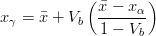 | (1.1) |
where is the average carbon content of the alloy, xγ is the carbon content of the austenite, and xα is the final carbon content of the ferrite, which can often be assumed to be negligibly small.
A plate (or sub–unit) of bainite forms with supersaturation of carbon which is then rejected into the residual austenite. The next plate of bainite then has to grow from the carbon enriched austenite. This process must cease when the austenite carbon concentration reaches the T0 curve, since nucleation of the next ferrite plate is thermodynamically unfavourable. If the reaction occurred with diffusion, the ferrite should continue to grow until the carbon para–equilibrium carbon concentration and the transformation would then go on until the carbon concentration of austenite reached the Ae3 curve.
The consequences of the T0 curve are that greater volume fractions of bainite can be achieved by transformation at lower temperatures, and that equilibrium carbon concentration of austenite given by the Ae3 curve cannot be reached, as is observed experimentally. The remaining austenite is available for further transformations, or can be retained after the sample is cooled to room temperature. The austenite can also be present both in the form of large volumes were little bainite has formed ‘blocky austenite’ and as thin films between the bainitic ferrite plates. The final form of the retained austenite is important for the mechanical properties of the steel, both the morphology and the composition, which effects the susceptibility and the consequences of further transformation to martensite during deformation.
Le Houillier et al. studied steels in which cementite precipitation was prevented, they suggested that a strain energy term should be included in the critical Gibbs energy for the bainite transformation [44]. Bhadeshia and Edmonds estimated the effect of strain and interfacial energy as 270 J mol−1 and denoted the calculated line T0′ [45, 46]. Later Bhadeshia took data from Steven and Haynes [47] and calculated the Gibbs energy for the ferrite and austenite at the BS temperature, and found that the value for the strain energy should be 400 J mol−1 [48].
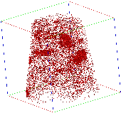
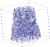
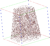
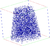
The diffusion rate of carbon in steel is many orders of magnitude greater than that for substitutional elements, meaning true equilibrium is unlikely to be reached at a transformation interface, especially as the temperature is reduced. The concept of paraequilibrium calculation was introduced, defined as a constrained equilibrium with carbon being able to diffuse freely but without change of any of the solute elements [49]. This is reasonable in many cases, because the diffusivity of carbon can be many orders of magnitude faster than solute diffusion or self–diffusion of iron. The bulk substitutional element content of bainitic ferrite has been shown to be identical to the parent austenite in atom probe experiments by Bhadeshia and Waugh [50, 51], Stark et al. [52, 53] and Josefsson and Andren [54] consistent with a displacive transformation mechanism.
Irvine and Pickering [56], and Shackleton and Kelly [57] observed bainite crystallography using electron diffraction, the crystallographic relationship between the ferrite and carbide components of bainite strengthened the concept that carbides in upper bainite precipitates from carbon enriched austenite, whereas carbides in lower bainite precipitate form from supersaturated ferrite plates (figure 1.7). Pickering [58] showed that both upper and lower bainite can occur during isothermal transformation at the transition temperature.
Matas and Hehemann [59] proposed that the transition from upper to lower bainite was decided by the time taken for carbon to partition compared to the time taken to precipitate carbides within the ferrite. Upper bainite forms at higher temperatures where carbon can partition to the austenite before it can precipitate in the ferrite. Takahashi and Bhadeshia [55] produced a quantitative model for the transformation comparing the time required to decarburise a super–saturated plate against cementite precipitation kinetics.
As we would expect lower bainite is more likely to form in high carbon alloys, and upper bainite more likely in lower carbon alloys. Not only is there more carbon to precipitate, but higher carbon contents mean that transformation is delayed to lower temperatures in continuously cooled samples. Srinvasan and Wayman [60] found that lower bainite formed at the bainite start temperature (BS) in a Fe-1.1C-7.9Cr wt% alloy and Ohmori and Honeycombe [61] showed that in high purity Fe–C alloys lower bainite is not obtained when carbon concentration is less than around 0.4 wt%.
Ko and Cottrell [62] studied the bainite transformation in situ using hot stage microscopy and reported surface relief similar to martensite. Growing plates also stopped when they reached austenite grain boundaries, which is not necessary for reconstructive transformations. Surface relief is consistent with a displacive transformation mechanism, while the observed slow growth rates support the idea that transformation is controlled by diffusion.
Oblak and Hehemann [34] rationalised the seemingly contradictory observations after studying the microstructures formed using electron microscopy, and observing that the microstructural unit was smaller than previously accepted. The apparent slow growth rates at the macroscopic scale could now be attributed to the growth of bainite by the repeated nucleation of ‘sub–units’, each of which grows rapidly to a limited size. The features which were thought to be plates were actually ‘sheaves’ [63] or ‘packets’, aggregate structures made up of these smaller sub–units or platelets. Figure 1.8 is the schematic representation of structures observed. The ‘macroscopic’ growth rate of the sheaf is therefore slower than the martensite transformation because it is largely controlled by the nucleation rate of these sub–units, although they transform by a martensitic mechanism, each one forming an acicular parallel plates around 0.2-0.5 μm in width and 1-10 μm in length.
Greninger and Troiano measured the crystallographic orientation of austenite and showed that the habit planes of bainite and martensite are both irrational, and that the habit plane of bainite is different from that of martensite in the same steel [64]. The habit planes varied with carbon content and transformation temperature. Observing that the habit plane of bainite approached that of Widmanstätten ferrite at high temperatures and that of proeutectoid cementite at low, Greninger and Troiano proposed that bainite grew from the beginning as an aggregate of ferrite and cementite, with competition between the two controlling the habit plane.
Smith and Mehl [25] later showed that the orientation relationship between bainitic ferrite and austenite does not vary greatly with varying carbon content or transformation temperature, and that it is similar to that for martensite and Widmanstätten ferrite, but dissimilar to pearlitic ferrite/austenite. Using pole figure analysis they determined that bainite had a Nishiyama–Wasserman [65, 66] relationship at 450 and 350∘C but bainite transformed at 250∘C and martensite had a Kurdjumov-Sachs [67] orientation relationship. Pickering showed that adjacent platelets in a cluster have almost identical crystallographic orientation [58], and are often found to be touching, separated by low–angle boundaries. Observing that this could lower the stored energy in the microstructure, and help to stabilise the structure against tempering. Davenport also reported the relationship could be loosely described as the Kurdjumov-Sachs type [68]. Crosky et al. [69] showed the orientation relation between the BCC and FCC phases after transformation are always found to be close to but never exactly the Kurdjumov–Sachs or Nishiyama–Wasserman orientation.
Kurdjumov–Sachs orientation relationship
{111}γ||{011}α
 γ||
γ|| α
α
Nishiyama–Wasserman orientation relationship
{111}γ||{011}α
 γ ≈ 5.25∘ from
  α towards
  α
α
Greninger–Troiano orientation relationship
{111}γ ≈ 0.2∘ from {011}
α
 γ ≈ 2.7∘ from
  α towards
  α
α
The relative orientations of the bainitic ferrite to the parent austenite have since frequently been found to be consistent with it being the Kurdjumov–Sachs or Nishiyama–Wasserman relationships, although neither is ever exactly matched. The two relationships differ by a rotation of about 5.25∘ about the normal to the parallel close–packed planes of the two structures. In martensite the relative orientation is found to be intermediate and irrational as predicted by crystallographic theory [19].
A high accuracy is required to compare theory with experiment, in bainite and martensite the required accuracy is difficult to achieve because of the experimental difficulties of retaining austenite and also the high dislocation densities. However experimental data always lie within the ‘Bain region’ which encompasses the Kurdjumov–Sachs and Nishiyama–Wasserman relationships [19]. The Bain region is defined as a result of the lattice deformation, which can be factorised into two components; the Bain strain which is the pure part of the lattice deformation, and a rotation of not more than 11∘ [19]. During the Bain strain no plane or direction is rotated by more than 11∘ since the two possible rational relations differ by a relative rotation of 5.25∘ about the normal to the parallel close–packed planes. This need not be the case for reconstructive transformations. For example allotriomorphic ferrite is known to grow into austenite grains with which it has an orientation which is random, or outside the Bain region, while during austenite grain boundary nucleation grows in orientation that is close to Kurdjumov–Sachs or the Nishiyama–Wasserman relationship [19].
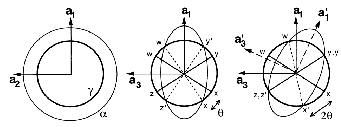
The face–centred cubic structure of austenite can also be described by a body–centred tetragonal unit cell, which can be converted to the body–centred tetragonal structure of martensite or to a body–centred cubic structure by contraction and expansion of the cell parameters. These deformations were first proposed by Bain and are known as the Bain strain [70]. Figure 1.9 shows the equivalence between the body–centred tetragonal (BCT) and face–centred cubic structures.
Although the Bain strain would produce the necessary change in crystal structure the macroscopic shape change would not be the same as the observed shape change, there is a further condition for a displacive transformation, that is the movement of a glissile interface through the parent phase. Wechshler et al. [71] and Bowles and Mackenzie [72, 73] developed a crystallographic theory to explain the transformation based on the movement of a glissile interface between the parent and product phases, and is consistent with the observed shape change.
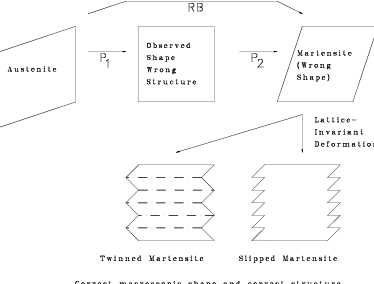
A pure deformation can be combined with a rigid body rotation to give a net lattice deformation which leaves a single–line undistorted, figure 1.10. However it is not possible to make a rotation that leaves two non–parallel lines undistorted so it is not possible to have an invariant–plane strain. This means it is impossible to have an interface between austenite and ferrite which is fully coherent and stress free, or transform between the phases with a strain that is an invariant–plane strain. To compensate for this discrepancy it is necessary to introduce a lattice–invariant deformation such as twinning of slipping as shown in figure 1.11. Such a substructure of twins or of slip steps is observed experimentally in martensite.
Displacive or martensitic transformations (e.g. transformation to martensite and bainite) conform to the phenomenological theory of martensite crystallography [72, 73]. Each of the requirements follows as a consequence of an invariant–plane strain deformation or the absence of substitutional atom diffusion.
Points 3, 4, 5 do not apply to face–centred cubic → hexagonal close–packed transformations.
The similarity between the bainitic and martensitic transformations is long established [22] and received added emphasis when is was shown that both transformations exhibit surface relief [62].
Hull [74] and later Bilby and Christian [75] proposed that martensitic transformations can be distinguished experimentally by means of the change in shape of the transformed regions. Christian also commented that surface relief does not necessarily result from non–diffusional transformation [76], and can also result in cases were the solute atoms can diffuse orders of magnitude faster than the solvent. Therefore surface relief cannot tell us if a displacive transformation takes place with or without carbon diffusion, however it is a necessary feature of martensitic transformation because of the lattice correspondence between the parent and product phases. Martensite, bainite, and Widmanstätten ferrite all exhibit a surface relief, with martensite transformation taking place with no carbon diffusion and the Widmanstätten transformation being controlled by carbon diffusion.
Surface relief when characterised as an invariant–plane strain with a large shear component can be taken to signify that the transformation mechanism involves the cooperative transfer of atoms from the parent to the product phase in a manner characteristic of shear transformations. The surface relief should be invariant–plane strain as in martensite, and has been characterised as having a shear strain component of 0.22 and a volume strain of 0.03 on transformation [77].
During transformation, one crystal grows at the expense of another by the migration of the interface. Christian [76] has said that a shape change in the transforming region can be expected for an appropriately coherent boundary between the parent and product phases of the martensitic type, provided the correspondence is not destroyed by diffusion. Assuming the crystals on each side of the boundary remain in contact, and remain coherent as the boundary moves, then any macroscopic shape change must be an invariant–plane strain on the plane at the boundary, or must differ from it only by strains that can be accommodated elastically in the vicinity of the boundary.
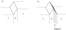
The strain energy for bainite when the shape change is elastically accommodated has been calculated to be about 400 J mol−1 [21], although there is the possibility that some of the strain can be relaxed by plastic deformation. One consequence of plastic deformation during or after transformation is the plastic yielding of austenite at the surface. Figure 1.12 shows the typical effects of the invariant–plane strain. The strain is followed or accompanied by a plastic relaxation in the austenite, resulting in a distinctive shape.
The transformation strain is a combination of the Bain strain and a rigid body rotation; it is an invariant–line strain. A further inhomogeneous lattice–invariant deformation, by shear or twinning, makes the transformation strain macroscopically an invariant–plane strain. The invariant–plane is also known as the habit plane. Figure 1.13 shows the nature of the invariant–plane strain, while experimental results are summarised in table 1.3 for different microstructures.
Swallow and Bhadeshia measured the surface topography using atomic force microscopy [77] and concluded that the relief of each sub–unit conformed with the general features of an invariant–plane strain. Whereas the nature of the shape deformation of Widmanstätten ferrite and martensite can be observed in the optical microscope, the bainite sub–units cannot because they are on a much finer scale. Atomic force microscopy is capable of resolving the bainite sub–units, the value of the shear component measured using light microscopy is around 0.13 [60, 78]. Theoretical predictions of the shear lie in the range 0.22-0.28 [77]. Measurement of the displacement of twin boundaries following transformation observed in the transmission electron microscope gives a value of 0.22 [79].
| Transformation | s | δ | Morphology | Reference |
| Widmanstätten ferrite | 0.36 | 0.03 | Thin Plates | Watson and McDougall [80] |
| Bainite | 0.22 | 0.03 | Thin Plates | Sandvik [81] |
| Bainite | 0.26 | Thin Plates | Swallow and Bhadeshia [77] | |
| Martensite | 0.24 | 0.03 | Thin Plates | Dunne and Wayman [82] |
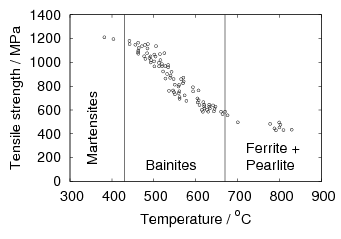
In general the strength of steels can be increased by lowering the temperature of the austenite to ferrite transformation [58], as shown in figure 1.14 lowering the transformation temperature usually increases the intensity of all the strengthening mechanisms. It is generally true that lower temperature results in finer grain size of the transformation product, greater dislocation density, finer dispersion of precipitated phases, and greater retention of solute in supersaturated solution. The results of Pickering [58] show a linear relationship between the transformation temperature and the strength over a wide range of bainite transformation temperatures, Davenport and Bain reported similar results for hardness after isothermal transformation [22]. It is also observed that upon continuous cooling fully martensitic steels can generate higher strengths than bainitic steels, usually tempering is performed on these martensitic steels to reduce the strength so as to provide adequate toughness prior to use.
Early bainitic steels were found to not be generally better in terms of mechanical properties than quenched and tempered martensitic steels due to the large size of the carbides, and the extra difficulty in implementing isothermal transformation. Irvine and Pickering introduced low carbon steels alloyed with boron and molybdenum [83] which delayed the pearlite transformation but maintained sufficiently fast bainite transformation kinetics, to allow production of fully bainitic steels by continuous cooling heat treatment. Later, higher cooling rates were introduced by using a laminar water jet system [84], and leaner alloys could be produced with higher strengths, leading to the development of High–Strength–Low–Alloy steels [85]. Relative to martensitic steels, the bainite microstructure is more stable upon further heat treatments, and bainitic steels have also been developed as creep resistant steels, for example composition Fe-0.1C-2.25Cr-1Mo wt% which exhibits excellent creep strength and microstructural stability [86]. Although the details of the microstructure may not have been known at the time it is now known to be a carbide–free upper bainite [19].
It is also known that addition of silicon or aluminium can prevent cementite precipitation during the bainite transformation. This is due to the high penalty of having silicon present in the cementite structure. In high silicon steels large carbides, which can lower the toughness of steel are prevented and the bainite plates are separated by thin films of retained austenite as have been studied by Bhadeshia and Edmonds [45].
Important classes of steels have been developed to take advantage of retained austenite to provide extra sources of plasticity. Transformation induced plasticity (TRIP) and TRIP–assisted steels [87, 88, 89], multi–phase steels (so called dual–phase steels), and more recently still, twinning induced plasticity (TWIP) aided steels [90, 91]. TRIP was first observed in heavily alloyed austenitic stainless steels, during deformation above their martensite start temperature. Matsumura reported the potential of TRIP–aided carbide–free steels, where carbon enrichment in the austenite resulting from transformation was used to stabilise the austenite. This greatly reduced the price of the stabilisation, and the effect could then be used to enhance the ductility of cold–formed high strength steels for automotive applications. In dual phase steels, inter–critical annealing replaces full austenitisation, in this case transformation to bainite takes place from a mixture of ferrite and austenite. For the same composition this may result in a greater amount of retained austenite, present in more refined regions.
The bainite transformation has been utilised to achieve areas of austenite of sufficient enrichment of carbon that they are stable enough to be retained in the microstructure, but are available for transformation upon deformation. In these TRIP–assisted steels the presence of retained austenite allows the strain–hardening rate to be decreased, or maintained to higher elongation. The ability of bainitic steels to produce retained austenite in the final microstructure has allowed a greater manipulation of the resultant mechanical properties.
This thesis describes the characterisation of a remarkable new bainitic steel, which
exhibits very high strength and hardness in bulk samples. The bainitic structure
which forms at low temperature in these high–silicon high–carbon steels offers
unique combination of mechanical properties, with strength of up to 2.5 GPa and
a toughness up to 28 MPa , depending on transformation temperature,
reported by Garcia-Mateo et al. [2].
, depending on transformation temperature,
reported by Garcia-Mateo et al. [2].
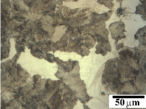
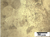
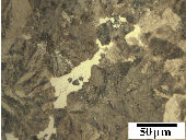
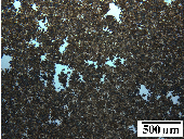
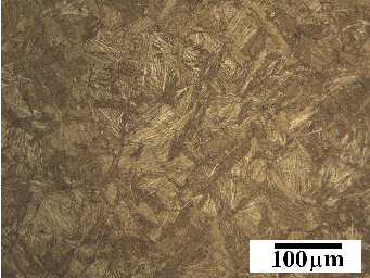
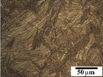
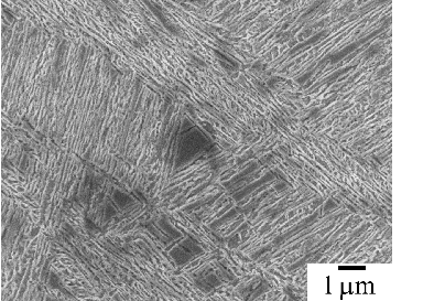
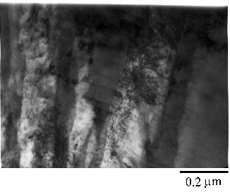
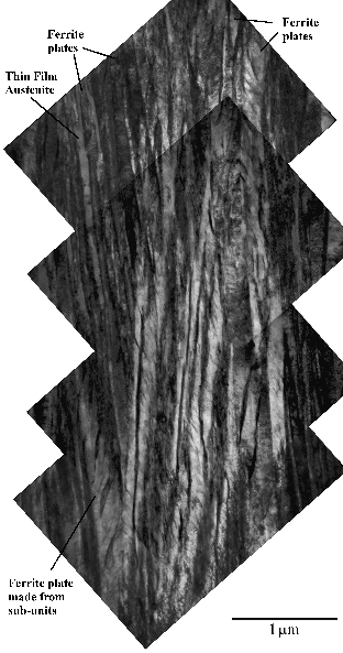
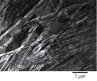
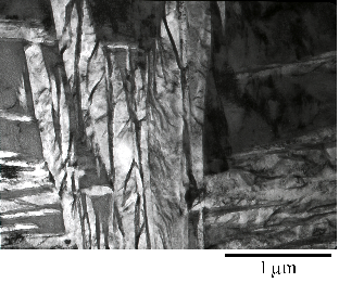
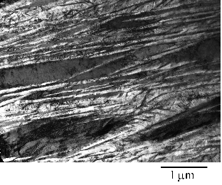
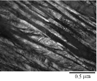
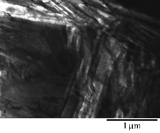
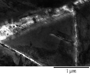
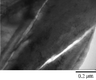
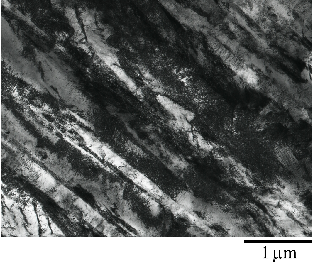
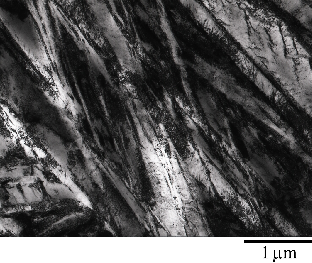
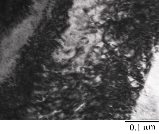
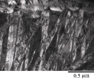
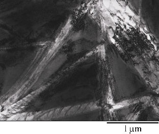
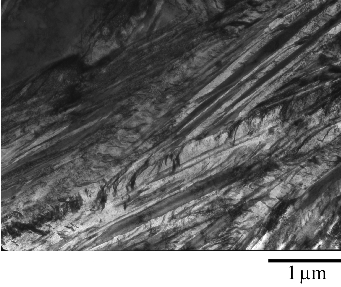
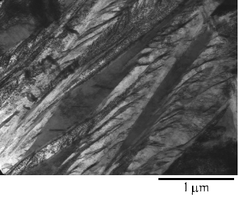
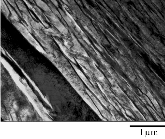
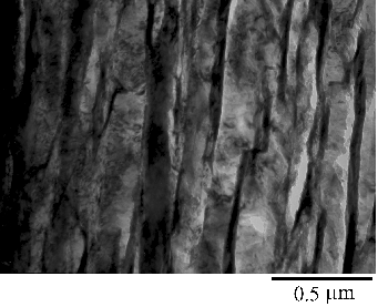
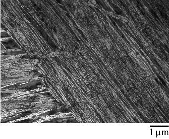
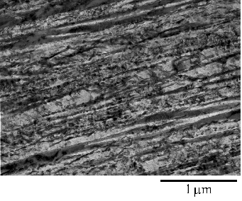
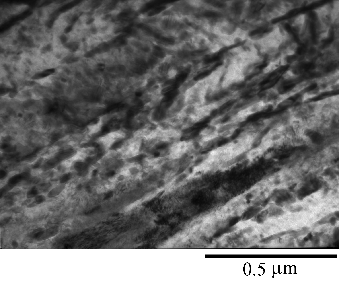
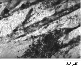
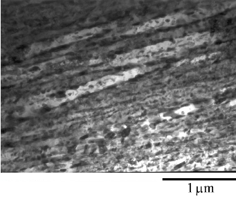
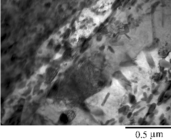
These mechanical properties are a result of a highly refined bainitic microstructure as shown in figure 1.15, due to transformation from austenite at temperatures of around 200∘C. Embrittling carbides are negated by the silicon additions. The microstructure then consists simply of plates of bainitic ferrite separated by thin films of austenite, the scale of both being unusually fine. Ferrite plates are reported to have widths of 20 nm compared to the usual width of 0.2 to 0.5 μm. Large regions of ‘blocky’ retained austenite which would otherwise limit the toughness could be avoided by maximising the volume fraction of ferrite, by transformation at the reduced temperature.
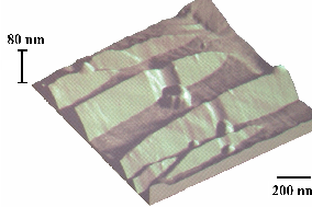
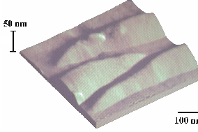
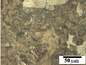
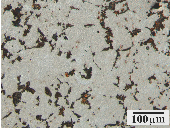
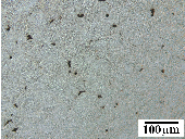
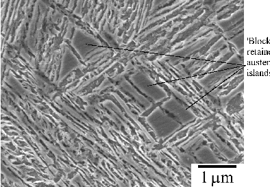
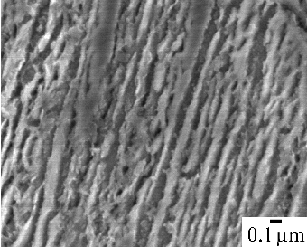
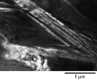
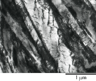
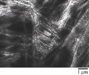
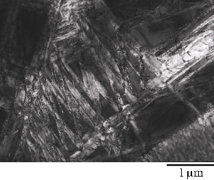
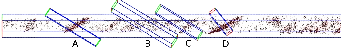
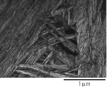
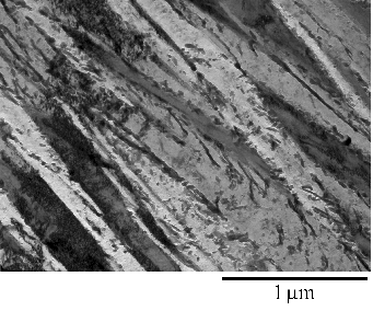
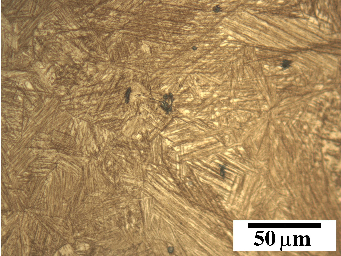
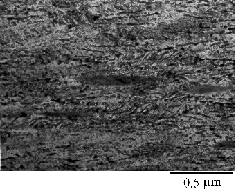
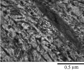
On a coarser scale the microstructure resembles wedge shaped sheaves of bainite (clusters of fine bainite plates separated by thin films of austenite when viewed at higher resolution) and small blocks of residual austenite, as shown in figure 1.16.
Transformation at low temperature not only results in high volume fraction of ferrite, but also leads to high strength by introducing a high number of defects into the microstructure. The defects take the form of dislocations and grain boundaries. The high dislocation density in the bainitic ferrite results in a huge supersaturation of carbon in the ferrite after transformation. It therefore seems remarkable that the hardness is also observed to be resistant to harsh heat treatments.
Caballero et al. [3] were the first to report transformation of high–carbon high–silicon steels at low–temperatures could result in nanoscale microstructure and result in extremely high strength steels. The discovery resulted from the investigation into the design of mixed microstructures of bainite and martensite to be produced from continuous cooling in medium carbon steels (e.g. Fe-0.3C-1.51Si-1.42Cr-0.25Mo-3.53Ni, Fe-0.32C-1.45Si-1.97Mn-1.26Cr-0.26Mo-0.1V) [94, 95]. Those steels have predominantly a bainitic microstructure consisting of fine plates of upper bainitic ferrite separated by thin films of stable retained austenite. Thermodynamics were utilised to design alloys so as to maximise the volume fraction transforming to the fine bainite structure, to avoid the large areas of retained austenite detrimental to toughness, by shifting the T0 curve to higher carbon contents, and by minimising the average carbon content [94].
Toughness values of nearly 130 MPa were obtained along with
strength in the range 1600-1700 MPa; these values match the critical
properties of marageing steels which are at least 30 times more expensive
to manufacture due to high alloy content of cobalt and nickel [95]. The
properties are also superior to quenched and tempered martensitic steels,
dual phase steels and TRIP-assisted steels as shown in figure 1.17. The
microstructure is resistant to tempering up to the transformation temperature,
however tempering at higher temperatures lead to the decomposition
of the austenite into ferrite and carbides, lowering both strength and
toughness.
were obtained along with
strength in the range 1600-1700 MPa; these values match the critical
properties of marageing steels which are at least 30 times more expensive
to manufacture due to high alloy content of cobalt and nickel [95]. The
properties are also superior to quenched and tempered martensitic steels,
dual phase steels and TRIP-assisted steels as shown in figure 1.17. The
microstructure is resistant to tempering up to the transformation temperature,
however tempering at higher temperatures lead to the decomposition
of the austenite into ferrite and carbides, lowering both strength and
toughness.
Microprobe analysis was used to determine the composition of the retained austenite and to investigate the properties of the austenite a steel was produced with the same composition: Fe-0.80C-1.60Si-1.99Mn-1.29Cr-0.25Mo-0.1V [98] (alloy A in this thesis). Although present as retained austenite within the bainitic microstructure, the composition was found not to produce a stable fully austenitic structure when in the bulk form [3, 98], with transformation to martensite taking place at around 120∘C. Subsequent experiments revealed that the steel could be transformed isothermally to bainite at temperatures as low as 125∘C.
Isothermal transformation experiments were conducted at 125, 150, 190, 250 and 300∘C, using hardness and optical microscopy to follow the progress of transformation and also using X–ray diffraction to quantify the volume fractions transformed. Bainitic microstructures with hardness around 600 HV could be produced by transforming at temperatures of 190 and 250∘C. These microstructures consist of around 60-70% of bainitic ferrite, with a plate size of around 50 nm separated by films of retained austenite which were even thinner [3]. The bainite transformation had a separate C–Curve on the TTT diagram with a well defined bainite start temperature as shown in figure 1.18.
Transformation to predominantly bainitic microstructures at similar temperatures has previously been reported by Davenport and Bain as early as 1930 [22], to temperatures as low as 140∘C as we saw figure 1.5. Although not reported it is probable that these microstructures contained large cementite particles due to the lower silicon content compared to the steels of Caballero et al.. However it may be noteworthy that Davenport and Bain did observe that austenite could be retained in the microstructures after transformation at low temperatures (140∘C) in some steels when the microstructure was bainite (referred to as martensite–trootsite in their paper) but only trace amounts were observed after transformation to martensite. Transformation at 180∘C resulted in a hardness of 62 Rockwell C (≈745 HV 2 ) and 64 Rockwell C (≈800 HV) at 140∘C along with 20-25 % retained austenite in Fe-1.13C-0.30Mn-0.17Si wt% alloy. An Fe-0.78C-0.36Mn-0.16Si wt% alloy achieved a hardness of 56.5 Rockwell C (625 HV) at a transformation temperature of 180∘C, this steel was the only one in the study which retained austenite after transformation at 180∘C.
All of the alloys studied by Davenport and Bain also had relatively fast transformation kinetics for diffusional products at higher temperatures, many of the transformation curves touching the axis at higher temperatures. Despite the fast cooling rates achievable by quenching into tin. It is possible that their hypereutectic steels would form cementite along the grain boundaries, which could have a devastating effect on toughness and the elongation in tensile tests. It is not known if Davenport and Bain pursued any further transformation experiments at low temperatures, since their main aim in this work seemed to be the classification of microstructures, and their work turned up many fruitful avenues of research.
Sandvik has previously studied the isothermal transformation in high–carbon high–silicon steels to bainite at 380∘C [100]. The steels of composition Fe-0.99C-2.21Si-0.78Cr-0.48Mn-0.017P-0.016S-0.035Al and Fe-0.91C-2Si-0.42Cr-0.59Mn-0.017P-0.031S-0.032Al wt% reporting that the steels exhibited a two stage transformation. Initially transformation rates were fast, followed by slow decomposition by formation of triclinic carbide and decomposition of the remaining austenite to ferrite. Sandvik attributed the delayed reaction of the second transformation as to it being governed by diffusion of carbon. The triclinic carbide is related closely to cementite, and due to the crystallographic relationships, crossings between carbide plates, and faulting on the (010)C planes it is thought the carbide forms by a shear mechanism.
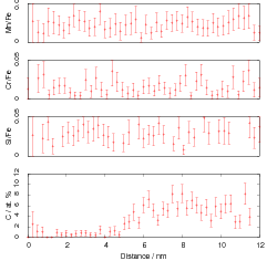
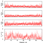
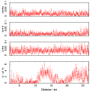
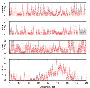
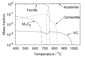
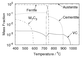
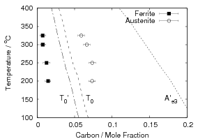
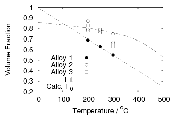
Garcia-Mateo et al. transformed steel of composition Fe-0.98C-1.89Mn-0.26Mo-1.26Cr-0.09V<0.002P (alloy B) at a range of temperatures and used X–ray diffraction to measure the carbon content of austenite and ferrite from the lattice parameter as shown in figure 1.19. The values indicated that there is high supersaturation of carbon in the ferrite and the level of carbon in the austenite determined in this way is higher than expected from calculation of T0’. One exception to the expected trend is that the level of enrichment of carbon in austenite is no higher than when transformed at 200 than 250∘C.
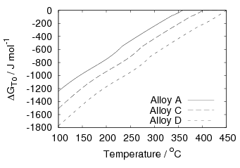
Garcia-Mateo et al. [102] then performed a series of thermodynamic calculations to see the effect of varying composition upon transformation kinetics, for the design of further alloys. A series of alloys were also produced to investigate the effect of various alloying elements. Comparison of the transformation kinetics against those calculated considering thermodynamics, as shown in figure 1.18 is very useful for design of further alloys. Garcia-Mateo calculated the effect of the different alloying elements, table 1.4 using thermodynamic calculation after Bhadeshia [48] and proposed further alloys with ferrite stabilising elements cobalt and aluminium to supply extra driving force for the transformation to bainite [103]. The characteristics of these alloys of composition Fe-0.83C-1.57Si-1.98Mn-0.24Mo-1.02Cr-1.54Co (alloy C) and Fe-0.78C-1.49Si-1.95Mn-0.24Mo-0.97Cr-1.6Co-0.99Al (alloy D) were reported in a series of papers [103, 104, 105, 106]. Figure 1.20 shows the difference in the driving force for transformation between the two alloys and alloy A.
| Element | Range in alloys | Effect on
| ||
| produced | T0 | BS | MS |
|
| C | 0.79–0.98 | — | ↓ | ⇓ |
| Si | 1.29–1.67 | ↓ | — | — |
| Mn | 1.5–3.79 | ↓ | ⇓ | ↓ |
| Mo | 0.21–0.25 | ↓ | ↓ | ↓ |
| Cr | 0.92–1.33 | ↓ | ⇓ | ↓ |
| Co | 0–1.5 | ↑ | ↑ | — |
| Cu | 0–0.2 | ↓ | — | — |
| Al | 0–0.2 | ↑ | ↑ | — |
| W | 0–1.0 | ↓ | ⇓ | — |
| V | 0–0.1 | — | — | — |
| Ni | 0–0.005 | ↓ | ↓ | ↓ |
The new alloys achieved faster transformation into the low–temperature bainite microstructure, and similar hardness values were realised [103]. The time to complete transformation at 200∘C was reduced from 310 h in alloy A to 160 h with addition of cobalt in alloy C, and 80 h with addition of both cobalt and aluminium in alloy D. Further acceleration could be achieved by lowering the austenitisation temperature to achieve grain refinement of the austenite, using equilibrium thermodynamic calculations to transform at temperatures were a small amount of carbides were present at the austenitisation temperature.
Garcia-Mateo et al. [107] also investigated the applicability of the nucleation functions as previously applied by Bhadeshia [48, 108] and Ali and Bhadeshia [109] to describe transformation to bainite and Widmanstätten ferrite. The bainite start temperature in the novel low–temperature bainitic steels could be explained by the parameters which had been previously derived at higher temperatures. Bainite forms below the calculated T0’ temperature when; ΔGγ→α < −G SB and ΔGm < ΔGN. GN being a universal nucleation function, describing the nucleation rate of bainite or Widmanstätten ferrite as a function of temperature.
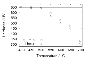
The plate size of the bainitic ferrite and the hardness were measured as a function of transformation temperature in alloys C and D [103]. Figure 1.21 shows the trend of hardness as related to plate size. A higher correlation was observed after calculating the area of interface per unit volume, SV , by accounting for the plate size and the volume fraction of bainite forming. There is some indication that the plate size does not depend upon just the transformation temperature. The alloys were transformed after two different austenitisation temperatures, and the measured plate size was smaller following the austenitisation at the lower temperature, some confidence in these values can be taken in that the samples with smaller plate size have a higher hardness. Austenitisation at the lower temperature will mean that carbides are present during austenitisation, effectively decreasing the concentration of carbon in the bulk.
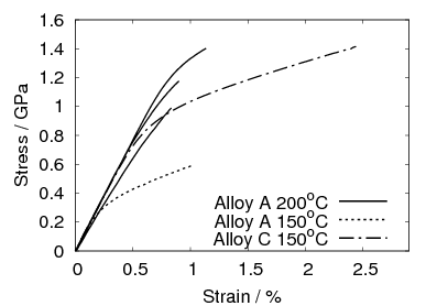
Mechanical properties and structure resulting from isothermal transformation
are summarised in tables 1.5–1.8 [3, 98, 4, 105] for the alloys with compositions
as shown in table 1.9. The tensile strength of the alloys C and D were measured
after isothermal transformation at 200, 250 and 300∘C [4], the stress–strain curves
for alloy C are shown in figure 1.22. In alloy C, transformation at 200∘C gave a
tensile strength of 2.15 GPa, with a yield strength of 1.4 GPa an elongation of 5%
and a fracture toughness (KIC) of 32 MPa . Transformation at higher
temperatures produces lower strength and greater ductility and toughness. In the
same alloy transformed at 300∘C the ultimate tensile strength was 1.8 GPa, yield
strength 1.3 GPa fracture toughness 45 MPa
. Transformation at higher
temperatures produces lower strength and greater ductility and toughness. In the
same alloy transformed at 300∘C the ultimate tensile strength was 1.8 GPa, yield
strength 1.3 GPa fracture toughness 45 MPa and elongation hugely
improved to 29%. The same trend was observed in alloy D, as shown in
table 1.8.
and elongation hugely
improved to 29%. The same trend was observed in alloy D, as shown in
table 1.8.
The carbon content in the bainitic ferrite was measured using X–ray diffraction, as was the dislocation density which was estimated from the peak broadening. It was noted that there was a correlation, and that the carbon enrichment increased with higher dislocation densities.
In alloy A it was observed that the carbon supersaturation in the austenite is no higher after transformation at 200 than at 250∘C. A similar anomaly in the levels of enrichment was also observed in alloys C and D. Rather than the expected trend of increasing austenite carbon content with lower transformation temperature, the opposite trend was observed as the transformation temperature was reduced from 300 to 250 and 200∘C. This was accompanied by lower elongation of the alloys transformed at lower temperatures, which could be related to the lower elongation by decreasing the stability of the austenite.
Garcia-Mateo [110] reported the strain hardening behaviour in the steels transformed at the different temperatures and calculated the austenite content as a function of plastic strain and composition after Sherif et al. [111]. Bhadeshia observed that the results show the amount of austenite at failure is usually around 10%, and related this to the percolation threshold. At around 10% of austenite it is no longer possible to have a continuous matrix and percolation of dislocations is no longer possible resulting in failure [112]. A similar value of the final austenite content for low–temperature bainitic steel has also been observed in the same steels by Sherif [96].
Hase et al. [113] transformed using a two–stage process, stepping the
temperature during transformation, this was able to achieve a higher amount of
retained austenite but avoid large blocks, and achieve a ductility of 40%,
toughness of 63 MPa and UTS of 1.5 GPa. Transforming at 250 and 350
resulted in similar strength level as transformation at 300∘C but better
elongation.
and UTS of 1.5 GPa. Transforming at 250 and 350
resulted in similar strength level as transformation at 300∘C but better
elongation.
| Alloy A | Temperature
| |||
190∘C | 200∘C | 250∘C | 300∘C |
|
| UTS / GPa |
| 2.00 | 1.93 |
|
| YS / GPa |
| 1.68 | 1.53 |
|
| TE |
| 3.1 | 8.8 |
|
KIC / MPa |
|
|
|
|
| Charpy VN / J |
| 4 | 6 |
|
| Hardness / HV20 | 650 | 650 | 575, 590 | 440 |
| Bainitic Ferrite C wt% | 0.32±0.07 |
| 0.32±0.07 | 0.20±0.07 |
| Bainitic Ferrite fraction | 0.87±0.01 |
| 0.84±0.01 | 0.65±0.01 |
| Plate thickness / nm |
|
|
|
|
| Austenite C wt% | 1.72±0.1 |
| 1.76±0.1 | 1.69±0.1 |
| Alloy C | Temperature |
|
||
200∘C | 250∘C | 300∘C | Ref. |
|
| UTS / GPa | 2.15 | 1.95 | 1.8 | [4] |
| YS / GPa | 1.4 | 1.5 | 1.3 | [4] |
| TE / % | 5 | 20 | 29 | [4] |
KIC / MPa | 32 | 38 | 45 | [4] |
| Hardness / HV20 (fine) | 660 | 589 | 500 | [103] |
| Hardness / HV20 | 690 | 640 | 490 | [103] |
| Bainitic Ferrite C wt% | 0.35 | 0.33 | 0.26 | [4] |
| Bainitic Ferrite fraction | 0.83 | 0.79 | 0.63 | [4] |
| Plate thickness / nm | 25 | 42 | 57 | [4] |
| Austenite C wt% | 1.1 | 1.4 | 1.49 | [105] |
| Alloy D | Temperature |
|
||
200∘C | 250∘C | 300∘C | Ref. |
|
| UTS / GPa | 2.2 | 1.9 | 1.7 | [4] |
| YS / GPa | 1.4 | 1.35 | 1.3 | [4] |
| TE / % | 8 | 9 | 29 | [4] |
KIC / MPa | 32 | 35 | 50 | [4] |
| Hardness / HV20 (fine) | 650 | 565 | 500 | [103] |
| Hardness / HV20 | 650 | 640 | 490 | [103] |
| Bainitic Ferrite C wt% | 0.35 | 0.34 | 0.29 | [4] |
| Bainitic Ferrite fraction | 0.87 | 0.79 | 0.74 | [4] |
| Plate thickness / nm | 45 | 42 | 53 | [4] |
| Austenite C wt% | 1.47 | 1.7 | 1.9 | [105] |
Alloy | C | Si | Mn | Ni | Cr | Mo | V | Al | Co | P | S |
A [3] | 0.79 | 1.59 | 1.94 | 0.02 | 1.33 | 0.3 | 0.11 | — | — | — | — |
0.98 | 1.46 | 1.89 | — | 1.26 | 0.26 | 0.09 | — | — | <0.002 | <0.002 |
|
C [4] | 0.80 | 1.59 | 2.01 | — | 1.0 | 0.24 | — | — | 1.51 | 0.002 | 0.002 |
D [4] | 0.78 | 1.49 | 1.95 | — | 0.97 | 0.24 | — | 0.99 | 1.60 | 0.002 | 0.002 |
Due to the high hardness the low–temperature bainitic steels have been investigated for use as armour steels, to replace more expensive armours. Hammond investigated the shock and ballistic properties to provide data for design of armour systems [114]. The strength of the material was found to be better when transformed at the lower temperatures, and can be as high as 10 GPa when the strain rate was 107 s−1 [115]. The armour systems developed from the material were found to be able to defeat the same projectile with a lower mass of armour, when compared against titanium and alumina armour systems [93].
Brown and Baxter criticised the commercial practicality of heat treatments lasting longer than 1 week, and also the cost of adding cobalt to accelerate transformation in these alloys, and claimed to solve these problems by altering the composition although they did not publish the full composition of the alloy they produced [98]. Transformation at 250∘C for 8 h, produced a microstructure with yield stress of 1673 MPa, UTS 2098 MPa and elongation of 8%. They also noted that all of the low–temperature bainitic steels have exhibited low values of Charpy impact toughness when tested at room temperature.
The cost of transforming steel for long periods of time at temperatures around 200∘C should not be expected to be costly in itself. The heat loss from a furnace increases with the operating temperature. For transformation of small samples in the laboratory small ovens are sufficient. For mass production, dedicated facilities are required, since it would always be un–economical to utilise a high temperature furnace which is needed for other applications. Temperature control within a few degrees may be necessary due to sensitivity of the plate size, transformation kinetics and volume transforming, and resulting mechanical properties to temperature.
To achieve very high strengths without introducing additional strengthening mechanisms, it may be unavoidable that long transformation times are needed, if the strengthening is mostly due to the plate size and the plate size is intimately related to the transformation kinetics. As transformation occurs by the repeated nucleation of sub–units, the transformation kinetics are determined by the time between nucleation events, and the volume of the sub–units transforming as a result.
Some models of bainite kinetics assume a constant volume for the sub–unit,
however attempts have also been made to account for the influence of
transformation temperature. There is little data on the volume of the plates, most
attempts have relied on using the plate width data of Chang [116]. Chester and
Bhadeshia modelled transformation kinetics of bainite transformation kinetics,
and showed that a better match could be achieved by considering the size of the
sub–unit. They used a linear relation, UW = 0.001077T − 0.2681, for the plate
width, and length of 10 μm, with a minimum plate width of 0.05 μm [117]. Parker
modelled the plate thickness using the equation 0.2 × (T − 528)∕150 μm. Matsuda
and Bhadeshia used this relation, with all the plate dimensions varying in the
same way, so the volume of the sub–unit varied as; V U = 2 × 10−17 × 3
m3 [118]. Matsuda and Bhadeshia assumed that in the initial stages of
transformation the volume of bainite is controlled purely by nucleation events at
the austenite grain surfaces, neglecting auto–catalysis, the volume of bainitic
ferrite is related to the grain boundary nucleation rate Ig, the volume of the
sub–unit V U, SV the austenite grain boundary surface area per unit volume,
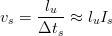
and time t since the start of transformation. After an initial stage they
then considered the lengthening rate of the sheaves of bainite vs to be
dominated by the time interval Δts between nucleation events after Ali and
Bhadeshia [119, 120].
3
m3 [118]. Matsuda and Bhadeshia assumed that in the initial stages of
transformation the volume of bainite is controlled purely by nucleation events at
the austenite grain surfaces, neglecting auto–catalysis, the volume of bainitic
ferrite is related to the grain boundary nucleation rate Ig, the volume of the
sub–unit V U, SV the austenite grain boundary surface area per unit volume,
and time t since the start of transformation. After an initial stage they
then considered the lengthening rate of the sheaves of bainite vs to be
dominated by the time interval Δts between nucleation events after Ali and
Bhadeshia [119, 120].
 | (1.2) |
Both of the nucleation rates for the sheave Is and grain boundary Ig are described by equations of the same form;
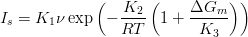 | (1.3) |
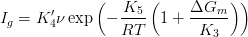 | (1.4) |
where Kn are constants previously derived [121, 122] or derived by Matsuda and Bhadeshia.
These equations treat the size of the sub–unit and the nucleation rate independently, but without a physical model to explain the limit to the plate size this cannot be confirmed. However it is clear to see that independently altering the plate size will proportionally decrease the transformation rate. In the equations presented, during the growth of the sheaves of bainite the growth rate depends only on the length of the bainite sheaf. Therefore long slender plates will be capable of growing quickly but still introducing a large area of interface per unit volume. As can also be seen, the nucleation rate can be increased via the driving force ΔGm which includes temperature and chemical effects.
If the effect is mainly due to the transformation temperature, it may be possible to achieve the same very fine plate size using more quickly transforming alloys, but of course there is a requirement to suppress the martensite start temperature sufficiently.
It would be beneficial to have a lower carbon variant, since high carbon steels are more difficult to weld. Bhadeshia demonstrated with calculations the difficulty of transforming at 200∘C in low carbon steels [123], this is because carbon is the most effective element at widening the gap between the martensite and bainite start temperatures (MS and BS). Alloying with nickel to suppress MS in a 0.1 wt% carbon 2 wt% manganese alloy depresses the BS temperature until it is lower than MS after around 5 wt% of nickel. Yang and Bhadeshia have made an experimental investigation of the possibility of low–carbon super–bainite, in a series of 0.1 wt% carbon steels, using nickel to suppress the martensite start temperature [124]. They found that the the bainite and martensite start temperatures are suppressed as expected, this might be useful for design of steels to be produced by continuous cooling, however they also reported that coalescence of the bainite plates occurred since there was an excess of free energy available at the BS temperature.
The magnitude of the different strengthening mechanism in low temperature bainite can be calculated based on the characterisation of the microstructure. Steel of composition Fe-0.8C-1.6Si-2Mn-0.3Mo-1.33Cr-0.1V transformed at 200∘C results in carbide free microstructure with a bainite plate size between 50 and 100 nm. X–ray diffraction experiments described later in the thesis reveal a large supersaturation of carbon in the ferrite.
If a stress is applied to a polycrystal, dislocations will first move in a grain having a large critical resolved shear stress. However, as dislocations cannot in general cross a grain boundary, they will pile up at the boundary until the stress there is sufficient to generate slip in an adjacent grain. At this point, general plastic flow can occur, and the material is said to have yielded.
For equiaxed grains the yield stress σy is related to the grain size d by equation 1.5, the Hall–Petch equation [125, 126, 127],
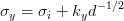 | (1.5) |
where σi and ky are constants, σi is sometimes called the friction stress.
Rhines [128] suggested that the physically significant parameter is the inverse grain boundary area SV rather than the grain size, equation 1.6. Naylor [129] and then Daigne et al. [130] demonstrated the inverse linear relationship for laths and plates as occur in martensite and bainitic steels, equation 1.7.
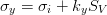 | (1.6) |
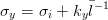 | (1.7) |
The strength of mixed microstructures of bainite and martensite was investigated by Young and Bhadeshia [131], they explained that a peak strength can be achieved in mixed microstructures by varying the combination of martensite and bainite. They described the strength with the equation 1.8 due to Bhadeshia [132]. The model was able to reproduce the trends and absolute values of experimental data of Tomita and Okabayashi [133, 134]. The strength of martensite and bainite was factorised into a number of intrinsic components. Mixed microstructures of bainite and martensite can be stronger than either of the individual phases, Tomita and Okabayashi suggest this is by effectively refining the austenite grain size by the bainite sheaves [135]. The peak strength of mixed microstructures can be explained by the model to be due to increased carbon in martensite forming from enriched austenite. The contribution from bainite at small volume fractions was larger than expected, this was attributed to a plastic constraint effect which enhances the strength of the bainite. It was found that an additional term was needed to explain the strengthening at low volume fractions of bainite, equation 1.9.
 | (1.8) |
where KL, KP and KD are constants, σFe is the strength of pure annealed iron, σss,i is the solid solution strengthening due to substitutional solute i, σC is the solid solution strengthening due to carbon, 3 is a measure of the ferrite plate size, and ρD is the dislocation density, δ is the distance between carbide particles, and the strength of constrained bainite may be represented by the equation,
![′
σB ≈ σB[0.65exp (− 3.3Vb) + 0.998] ≤ σM](superbainite51x.png) | (1.9) |
where σB and σ′B represent the strength of constrained and unconstrained bainite respectively, σM is the strength of martensite, and V b is the volume fraction of bainite. For a mixture containing 0.5 volume fraction of bainite this will increase the strength of the bainite component by 12%, and with 0.8 volume fraction will give an increase of 4.5%.
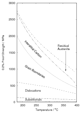
Garcia-Mateo and Caballero [4] reported the results of mechanical testing and allocated the strengthening to contributions from the plate size and the dislocation density. Dislocation density was measured from the peak broadening in X–ray diffraction experiments and plate thickness measured using transmission electron microscopy. The reported contributions are shown in figure 1.23 and compared against the 0.2% yield strength and the ultimate tensile strength.
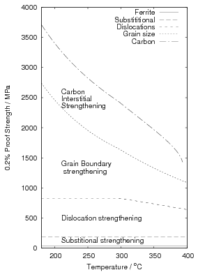
The strengthening contributions can also be calculated from equation 1.8 neglecting the effect of constraint, which for large volume fractions should account for around 4% increase according to equation 1.9. Using equation 1.8 allows calculation of the strength of the bainitic ferrite as a function of temperature, the result of which is shown in figure 1.24. It should be noted that from the previous results carbon supersaturation in the ferrite should be expected to make a large strengthening contribution, but has been omitted by Garcia-Mateo and Caballero.
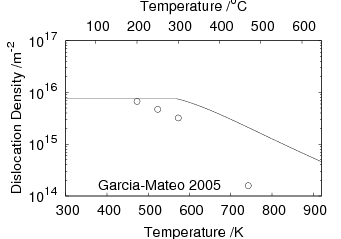
The dislocation density values reported by Garcia-Mateo et al. are in general agreement with the relationship proposed by Takahashi and Bhadeshia, as shown in figure 1.25. Takahashi and Bhadeshia showed the trend of increasing dislocation density with decreasing transformation temperature for both martensite and bainite, with a maximum dislocation density at around 350∘C [55]. Noting that the tendency for accumulation of dislocations by plastic deformation, and removal by recovery effects are both dependent largely on the transformation temperature they proposed the empirical equation 1.10. Dislocation density and therefore strength contribution is reasoned to be constant at lower temperature following Young and Bhadeshia [131]. For a given composition of bainitic steel the substitutional solute concentration in the ferrite is fixed, without precipitation of carbides the effect of transformation temperature will be via the grain size, dislocation density, and the carbon in the ferrite.
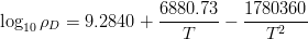 | (1.10) |
where ρD is the dislocation density, the length per meter cubed, and T is the absolute temperature in Kelvin.
The bainitic ferrite makes up only part of the microstructure, and this proportion increases with decreasing temperature, as volume fraction of ferrite increases as the temperature is decreased. This can be calculated by using thermodynamic calculation of the limiting T0 curve or can be empirically fitted to the volume fraction data reported by Garcia-Mateo et al..
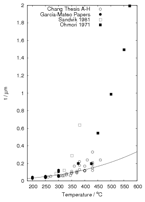
Garcia-Mateo et al. [92] reported values of carbon content measured by X–ray along with plate thickness in alloy B in the temperature range 200–320∘C. The plate size as a function of temperature can be calculated as a function of temperature using an arbitrarily chosen function fit to the plate width data provided by Garcia-Mateo. This was found to be a linear relationship on a log–log plot of plate size against temperature. Fitting to a larger data set of all the values reported in the literature was not trivial, not only are their problems performing regression due to bias by outliers, but it also seems that there is disagreement between the results of the different authors [100, 137, 116, 103], as shown in figure 1.26. While the values do tend to converge as the temperature is decreased, at higher temperatures there are very different values for the different steels studied by the various investigators. It is probable that there are also composition effects which would need to be accounted for in a physical model. Composition effects on the plate size have been previously investigated by Singh and Bhadeshia [138], who created a neural network model to account for the effects due to the strength of austenite and the chemical driving force available for transformation. The model shows that increasing the strength of the austenite by 100 MPa can lead to a decrease of 0.2 μm, this is thought to be consistent with plate size being limited by plastic deformation induced during transformation. For purely elastic deformation of the plates, the opposite trend should be expected, increase of plate size with the increased driving force available at lower temperatures [139].
Factor | Strength Contribution | Ref. |
Fe |
| [140] |
C | 0.25wt% C × 3700 MPa/wt% | [141] |
C | (0.25wt% C)1∕2 × 1722.5 | [142] |
C | (0.25wt% C)1∕3 × 1171.3 | [143] |
Si | 1.6 wt% Si × 85 MPa/wt% | [141] |
Mn | 2 wt% Mn × 32 MPa/wt% | [141] |
Mo | 0.3 wt% Mo × 30 MPa/wt% | [141] |
Cr | 1.33 wt% Cr × -30 MPa/wt% | [141] |
V | 0.1 wt% V × 9 MPa/wt% | [140] |
Dislocations | 7.34 × 10⁻⁶ × |
|
Plate Size | 115 ×
exp | |
Cementite spacing | Not applicable |
|
Using a rule of mixtures with a linear weighting of the volume fraction, the yield strength of low–temperature bainitic steels can be calculated, as shown in table 1.10 and figure 1.27 were the calculation is for alloy B. To make the calculation, fitting to experimental data has been used, although in principle the calculation can be made more physical, it may be misleading to base calculation on thermodynamics unless the levels of carbon supersaturation in austenite and ferrite and the volume fractions match the experimental values, which is not yet the case. Instead a series of empirical approximations were made to the reported values of plate size, volume fraction, and compositions of the phases.
An arbitrary linear fit was used to include the relationship between the volume fraction of bainitic ferrite and temperature. As shown in figure 1.28 this better matches the experimental measurements than the calculation based on thermodynamic T0. Values reported between 200 and 300∘C are approximately linear, and lower than thermodynamic calculation of same. The strength of the retained austenite was estimated to be 640 MPa, calculated using empirical equation after Irvine et al. for the enriched composition but ignoring any grain size effects [144]. Extrapolation of yield stress data from higher temperature tests [145] using a function for the strength as a function of temperature [138] gives an estimated yield strength of around 500 MPa at room temperature for the composition before enrichment, and agreed with the calculated value using the function of Irvine et al..
As shown in the figure, accounting for the volume fraction of bainitic ferrite makes the calculated yield strength much more sensitive to the transformation temperature than before. Not only is the bainitic ferrite harder, but the larger volume fraction makes a larger contribution to the final strength. It is also apparent that the strength of the austenite can only make a minor contribution to the strength unless it can have comparable strength as the bainitic ferrite.
The calculated yield strength is much higher than the strength realised in the low–temperature bainitic steels. This may be due to incorrect calculation of the strength of the bainitic ferrite, it may be more appropriate to omit the effect of carbon as Caballero and Garcia-Mateo, and only consider strengthening by dislocations and plate size, this would be the case if the carbon trapping in the bainite is of a different character to the trapping in martensite. It may also be that the details of the calculation are overestimating each of the strengthening effects due to extrapolation from the range of previous results.
This calculation considers only strengthening in the bainitic ferrite, there may also be strength contributions from austenite thin films which will be hard due to high carbon content. However it probably is not appropriate to treat the thin films and ferrite plates completely separately. Because the bainitic ferrite and austenite thin films form an intimate mixture, it may have been more appropriate in the calculation to treat this as a volume containing ferrite and austenite strengthened by the grain boundaries between them. Garcia-Mateo et al. noted that in practice the mean lineal intercept should depend upon the volume fraction of bainite as SV = V B∕t. The strengthening value used is for martensite existing without considering if thin films of austenite are present.
It is also possible that the calculation for the strength of the bainitic component is correct, and that yield strength and ultimate tensile strength of the mixture are determined to a larger extent by the mechanical properties of the austenite. In this case it may be that calculation by the rule of mixtures used here is too naive. In this case it may be that better calculation could be made by considering load partitioning in a composite of bainitic ferrite and austenite. This would be more reasonable since we expect the austenite has a lower strength than the bainite.
Nevertheless the calculation demonstrates the huge contributions to the strength that are possible by refining the microstructure to such a large extent.
It is not possible to strengthen by perfection in bulk materials, the ideal properties are only available on a very fine scale. Strengthening is therefore carried out by introducing large numbers of imperfections into the microstructure. There are practical limits to deformation that can be achieved meaning it is not possible to heavily deform large cross–sections. Therefore, as pointed out by Bhadeshia [123] displacive transformations have the greatest potential for grain refinement of bulk materials. Since the transformation causes the refinement in microstructure it is possible to transform in bulk to this heavily deformed microstructure.
The highest strength achieved in iron or steel would be for a such defect–free structure. The shear stress to plastically deform such a structure would be the stress to move one plane of atoms past another, this stress was first calculated in 1926 by Frenkel [146] assuming there is a periodic shearing force required to move the top row of atoms past the bottom row given by a sinusoidal relation:
 | (1.11) |
where τ is the applied shear stress, G is the shear modulus, a and b are the spacings between atoms between rows of atoms and in the direction of the shear stress, and x is the shear translation away from the low–energy equilibrium position. The maximum value of τ, is the theoretical critical shear stress;
 | (1.12) |
which can be approximated by τm = 0.11G since atomic theory shows that
inter–atomic forces peak at a strain of about 0.2. If the shear modulus of
body–centred iron is taken as G = 59 GPa, then the ideal shear strength will be
6.5 GPa. This means that the theoretical highest tensile strength achievable in
iron is 21 GPa [147], for a perfect ferrite crystal, under uni–axial tension in the
 direction.
Clatterbuck et al. [148] have made ab-initio calculations of the ideal strength
of iron in tension and shear. In  tension the ideal strength of 12.6 GPa was
determined by the elastic instability of the ferromagnetic phase along the ‘Bain’
strain path from body–centred cubic to face–centred cubic. The shear strength in
the
tension the ideal strength of 12.6 GPa was
determined by the elastic instability of the ferromagnetic phase along the ‘Bain’
strain path from body–centred cubic to face–centred cubic. The shear strength in
the  {112} and
  {110} shear systems was 7.2 GPa and 7.8 GPa largely
determined by the body centred tetragonal structure with the two shears
having slightly different paths from body–centred cubic to body–centred
tetragonal.
{110} shear systems was 7.2 GPa and 7.8 GPa largely
determined by the body centred tetragonal structure with the two shears
having slightly different paths from body–centred cubic to body–centred
tetragonal.
It is possible to get close to perfection in fibres of relatively small dimensions. Brenner [149, 150] performed tensile tests on defect–free whiskers of iron and reported a tensile strength of up to 13.23 GPa, and it is possible that this tensile strength was limited by dislocation nucleation from the free surfaces rather than by elastic instability.
The highest strength available in commercially available steel is 5.5 GPa in ‘Scifer’, which takes the approach of using severe deformation to introduce large numbers of defects into the material by mechanical deformation. Unlike perfect crystals, the strength of Scifer is not dependent on size, however the material is only available in the form of fine wires because of the practical limits of introducing the necessary deformation.
Figure 1.29 compares the strength of the perfect whiskers measured by Brenner, the commercial Scifer wire [151] and the mechanical properties achieved to date with the novel bainitic steels which are examined in this thesis.
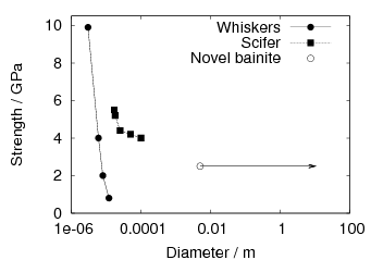
A unique feature of grain–size strengthening is that it also increases the toughness. In metals and alloys which undergo a ductile to brittle transition the transition temperature is reduced [152]. The impact transition temperature of ferrite can be described by an equation of the form βTD→B = ln β − ln C − ln d−1∕2 where β and C are constants, and TD→B is the ductile-brittle transition temperature, and d is the grain diameter. Therefore smaller grain sizes are highly sought after in industrial steel production.
Industrially thermomechanical processing of plain carbon steels can produce ferrite grain sizes between 5 and 10 μm, whilst laboratory tests have achieved grain sizes approaching 1 μm [153]. Yokota et al. [154] investigated the limits of the grain size refinement by considering the heat released during phase transformation. Since the latent heat released during transformation is known to cause recalescence, which is likely to limit the minimum size of the allotriomorphic ferrite grains. The size of which may depend upon the magnitude of the free energy change and the amount of energy stored as surface energy in the grain boundaries equation 1.13 [154].
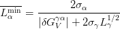 | (1.13) |
During adiabatic transformation the temperature will increase according to:
 | (1.14) |
where ΔT is temperature change in Kelvin, ΔH is the enthalpy change, Cp is the specific heat capacity, values of the finest achievable grain size where then calculated assuming that all the enthalpy change is used in heating the sample, and found to agree with experimental values.
One strategy to avoid recalescence due to the heat of transformation is to slow the transformation and decrease the difference in energies between phases. Table 1.11 shows the stored energy for different microstructures of steel, martensite has the highest amount of energy stored, followed by bainite. The strain energy due to the displacive transformation decreases the energy difference between the two phases, lowering the amount of heat generated during transformation, allowing a greater refinement of grain size. The temperature raise during transformation will also depend upon the rate of transformation and the rate of heat removal from the area transforming. This will depend upon thermal conductivity and rate of heat removal from the surface, so a second strategy could be to transform at a slower rate.
In the novel bainitic steels the transformation is carried out at a low temperature and the rate of transformation is slow. Since the rate of transformation is reduced the energy produced by the transformation has time to dissipate rather then increase the temperature of the material, helping to avoid coalescence of fine grained microstructure.
Coalescence is also known to take place during the bainite transformation, this is usually a feature of weld microstructures, and is thought to be associated with a reduced toughness [155].
Phase in Fe-0.2C-1.5Mn wt% at 300 K | Stored Energy / J mol−1 |
Ferrite, graphite & cementite | 0 |
Ferrite & cementite | 70 |
Paraequilibrium ferrite & paraequilibrium cementite | 385 |
Bainite and paraequilibrium cementite | 785 |
Martensite | 1214 |
Mechanically alloyed ODS metal | 55 |
Tempering heat treatments take place at temperatures were austenite decomposes and the metastable microstructure of steel approaches the equilibrium structure. The changes during tempering of martensite have been classified in stages, as shown in table 1.12. When martensite and bainite transformation occurs at higher temperatures it may be accompanied by many of the stage 1 reactions. In martensite this is called autotempering, in bainite it is often unavoidable due to the higher temperature of transformation.
Stage 1 |
Segregation of excess carbon to defects or clusters |
Precipitation as cementite, or transition carbides in high–carbon steels |
|
Stage 2 |
Most of carbon precipitates |
Carbides convert to cementite |
Austenite decomposes |
|
Stage 3 |
Spheroidisation/coarsening of carbides |
Recovery of dislocation structure |
Alloy carbide precipitation |
Recrystallisation of ferrite |
In martensitic steels the hardness and strength drop rapidly during tempering, as carbon leaves solid–solution. In contrast bainitic steels usually soften more slowly on tempering [21]. Usually the carbon supersaturation is much lower in bainitic steels, also the stored energy in the microstructure is lower than in martensite, decreasing the driving force available for coarsening. In quenched steels containing carbon above 0.4 wt% carbon, and in silicon containing bainitic steels austenite can be retained in appreciable quantities, the decomposition upon tempering has been shown to occur by a reconstructive mechanism [157].
Irvine and Pickering introduced a tempering parameter T(20 + log t), to allow estimation of the effect of time and temperature, using the kinetic strength concept introduced by Hollomon and Jaffe [158]. Although difficult to justify from a mechanistic point of view it was demonstrated to be useful in representing the hardness of bainite as a result of tempering.
In high–carbon steels it is usual to form transition carbides first on tempering of martensite, which transform to cementite up on further tempering. Transition carbides are also possible during isothermal transformation of high–silicon bainites in cases when the steel is not held for sufficient time to allow long range diffusion of substitutional atoms 3 .
Kalish showed that a dislocation densities of 2 × 1012 cm−2 could trap sufficient carbon to prevent 𝜖–carbide in martensite.
Silicon additions are also known to add to the resistance to tempering in martensitic steels [8, 9, 159]. In silicon–containing bainitic steels containing retained austenite, the decomposition of the austenite into a harder mixture of ferrite and carbides will compensate for some of the loss in strength of the ferrite.
Caballero et al. [3] observed that the low–temperature bainitic steel was remarkably resistant to tempering, maintaining the hardness after severe heat treatments as shown in figure 1.30.
Transformation of high–carbon high–silicon steels results in a carbide free microstructure of bainitic ferrite and austenite. The novel microstructure resulting from transformation at low–temperatures results in high strengthening attributed to the very fine scale of the bainite plates and the high dislocation density. The hardness of the microstructure has also been observed to be resistant to tempering, compared to similar strength martensitic steels which rely predominantly on carbon in solution to provide strengthening.
Uniquely, the very high strengths achieved do not necessitate any large deformations, or rely on perfection which is only available at very small scales, it therefore possible to transform large sections of material to this microstructure.
However the subject is not completely understood, or without problems. Industrially it may be viewed as a problem to take many days or weeks to perform a heat treatment, which may restrict the steels to only special applications. It is not known if the small scale is fundamental to transformation at low temperature. There is no explanation of the very fine scale of the microstructure, and how this differs from the formation of martensite.
It is therefore interesting both from a scientific viewpoint and industrially to examine the transformation and subsequent tempering behaviour.
Study of the surface relief was performed to quantify the magnitude of the shear component during the martensitic transformation of bainite. For martensite and Widmanstätten ferrite values can be obtained from optical microscopy, but in the case of bainite the plate size necessitates techniques capable of higher resolution.
Atomic force microscopy measures the topography of a sample by rastering a sharp tip, typically with radius less than 10 nm in diameter, across the surface. The tip is placed at the end of a cantilever and the displacement of the tip as it scans the surface can be measured by an array of photo-detectors which measure the deflection of a laser beam reflected from the back of the cantilever.
Samples were prepared from alloy A (Fe-0.79C-1.59Si-1.94Mn-1.33Cr-0.3Mo-0.11V wt%) by metallographic polishing, particular care was taken to prevent contamination of the surface with oil, after polishing to 1 μm the samples where cleaned with high purity ethanol. Samples were then sealed in partially evacuated quartz tubes flushed with argon, for austenitisation and transformation. Samples were either square cross section rod samples 4 mm × 4 mm × 30 mm with each face polished, or disc samples 3 mm in diameter 1-2 mm in depth. To combat oxidation of the surface titanium powder was added to the tubes separated by cotton wool to ‘get’ any oxygen remaining in the tube during furnace heat treatment. Specimens were austenitised for 15 min at 1200∘C before isothermal transformation allowing sufficient time so that the microstructure can be expected to be a mixture of bainite and austenite based on previous results.
A Seiko SPA-300 AFM was operated in contact mode with a 20 μm scanner table and a force reference of 1.95 nN. Images were acquired with 512 × 512 pixel resolution the maximum scan speed used for imaging was 1 Hz and this was reduced to prevent artifacts due to excessive ‘jumping’ of the tip caused by scanning over the surface. The voltage sensitivity for the vertical dimension (nm/mV) was calculated automatically based on the dimensions and resonant frequency of the cantilever which had been supplied by the manufacturer who measured the dimensions of each tip. The quoted accuracy of the frequency is 10%, resulting in 10% error in the measurement of the vertical dimension. Horizontal dimensions were not calibrated, however it is reasonable to believe that the errors from surface artifacts, and vertical calibration will be much larger than the error in measuring the horizontal dimensions. Piezoelectric sensors are not thought to significantly degrade during their lifetime. Placement of cross-section for profile measurement should only contribute a small error to the calculated width, this can be placed perpendicular to the axis of the plate with reasonable accuracy by eye. Some experiments were also performed with a digital instruments nanoscan AFM operated in non-contact mode.
Samples were also transformed and then examined in a focused-ion-beam microscope (FIB). In this experiment a platinum layer was first deposited on the surface, and the cross-section can be examined by milling a trench in the surface of the material using a focused beam of ions.
Figure 2.1 shows the surface relief formed due to the bainite transformation, at 200∘C for 7 days. The sheaves of bainite can be observed using optical microscopy, but the sub-units cannot be resolved. Since the grain boundaries are also visible due to thermal etching it can be observed that the sheaves grow until they impinge on each other, or reach a grain boundary. The sheaves do not grow across the grain boundaries that exist during their growth, consistent with previous observations, and as a result of the displacive transformation mechanism. Small blotches on the surface are presumably the result of oxidation.
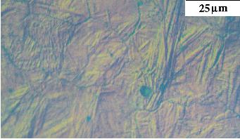
Figure 2.2 shows the surface relief caused by the displacive transformation. Both images are representations of the same 10 μm2 area, in the first the colour represents the height, the second image is a 3D representation of the surface. Ridge-shaped upheavals with a large aspect ratio can be seen, having lengths between 2 and 6 μm while being a fraction of a micrometre in width. The shape and distribution is similar to the bainite plates when observed at high magnification in an electron microscope. As will be seen in the other images the total width of the transformation upheaval of each sub-unit is around 200 nm wide. Other than the surface relief due to the sub-units, bright round patches can be seen. These are conical in the three dimensional images. This is thought to be due to oxidation or some other contamination of the surface. The samples tended to degrade with time, becoming more oxidised or contaminated, until the sub-units could no longer be seen.
The apparent shear component SA was determined by measuring the gradient of slopes from the foot to the tip of the slope (SA = height∕width). A decision was made which side was the shear due to bainite transformation and which was due to plastic deformation by looking at the shape of the plate, and by comparing adjacent plates when possible. The angle of shear of adjacent plates should be similar because they should have similar crystallographic orientation within a bainite sheaf. Otherwise a decision can be made assuming the shear is well defined in comparison to the plastic accommodation in the austenite. Figures 2.3 and 2.4 show the 3D representations of the areas scanned, and figures 2.5–2.7 shows the corresponding line scans. The measurements are summarised in figure 2.8.
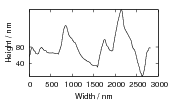
(a) Profile from Fig. 2.3a, SA=0.40, 0.39, 0.47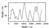
(b) Profile from Fig. 2.3b, SA=0.39, 0.39, 0.35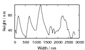
(c) Profile from Fig. 2.3a, SA=0.45, 0.39, 0.33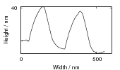
(d) Profile from Fig. 2.4b, SA=0.27, 0.29 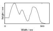
(e) Profile from Fig. 2.4b, SA=0.33, 0.24, 0.39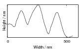
(f) Profile from Fig. 2.4b, SA=0.31, 0.24, 0.33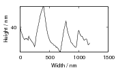
(g) Profile from Fig. 2.4a, SA=0.35, 0.43, 0.46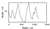
(h) Profile from Fig. 2.4a, SA=0.34, 0.32, 0,36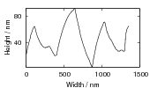
(i) Profile from Fig. 2.3c, SA=0.27, 0.30, 0.41
Looking at just the 3D representations and the line scans produced by the machines software can give an exaggerated view of the magnitude of the features, as demonstrated by comparing figures 2.4 (a) and (b). If the shear component is around 0.25–0.28 the features expected due to shearing should be 3.5-4 times wider than they are high, it may be more useful to interpretation of the data to plot the data with a 1:1 ratio between the scales of height and horizontal displacement, as demonstrated in figure 2.6 and 2.7.
The result of measuring the apparent shear is shown in figure 2.8 and 2.9, the sub–figure captions in figure 2.5 indicates were each reading was made. The average of the observations is 0.31, and the maximum 0.46, both numbers are higher than the expected maximum of 0.28 based on the values calculated from the phenomenological theory of martensite crystallography [77], and larger than the previous experimental observation of 0.26 [77]. The maximum value should be expected when the plate major axis is perpendicular to the surface. It is possible that the fine scale of the microstructure resulting from transformation at 200∘C means that the error in observation from surface roughness is larger, in this case we should expect a larger deviation around the average value. It is possible that roughness may also result in a sampling error due to the lower prominence of plates with lower SA.
Plotting the observed values against the plate width is a useful exercise to classify the results, as can be seen from figure 2.9. Larger features, which are more likely due to agglomeration of plates in sheaves, have lower apparent shear. The value is consistent with the previous observation of sheaves of bainite made by optical microscopy (0.13) [160, 78].
Complete elastic accommodation of the shear due to transformation should result in a surface step where as plastic accommodation in the austenite can occur, leading to relaxation of the surface. In contrast in Widmanstätten ferrite the shape change is partially accommodated by twinning, resulting in a tent-like surface relief. As can be seen in the cross–sections figures 2.5–2.7, in many cases the transformation at 200∘C did not result in a symmetrical surface relief features. Measurements of the ’Apparent shear’ of both slopes of the surface relief features are summarised in figure 2.10.
The angle of the plate to the free surface will also have an effect on the measurement.If h and w are the measured values of height and width of a plate the apparent shear is simply given by,
 | (2.1) |
Considering the orientation of a bainite plate intersecting with the free surface with angle 𝜃, if we re–orientate the plate onto the surface then the true plate width a and the height b would be given by,
 | (2.2) |
 | (2.3) |
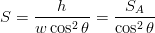 | (2.4) |
For grains intersecting at all angles between 0-90°with equal probability, the effect should be that the average SA is half the value of S, and the maximum value measured should be equal to S. This may explain the large difference between the previous workers values measured for sheaves of bainite and those measured on individual plates. However, the sheave of bainite will also include areas of untransformed austenite. It should also be considered that in measuring individual plates it is unlikely that we will distinguish plates orientated at very low angles to the surface, and perhaps more importantly it is possible that the sheaves have a preferential orientation at high angles to the surface, since this may allow a volume of material to transform in such a way as to and minimise the strain energy. The cost of creating extra surface area presumably is much lower. Therefore the greatest preference would be for a technique which allowed the measurement of both the surface relief at the necessary scale, and also the orientation of the plate below the surface.
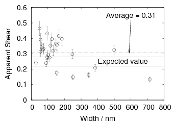
Observations of the microstructure were made using the focused beam ion microscope as shown in figure 2.11. Phase contrast on the flat surface could be achieved using the contrast in ion-beam imaging. It was not possible to resolve the microstructure using electron microscopy. With the resolution achieved it is not possible to measure the surface relief, but it does show that the plates and sheaves are orientated at high angles to the surface. If plates are always close to perpendicular to the surface, this would help to explain the consistently high apparent shear values, although not the magnitude being higher than 0.28.
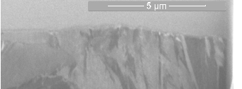
Theory predicts the shear on the surface should be in the range 0.22–0.28 [161, 137, 162]. The observation on the steel transformed at 200∘C suggests the shear component may be larger as a result of transformation at the lower temperature. This would be consistent with the observed long slender shape of the bainite plates if the elastic accommodation of the shape change is important during growth.
The small scale of the bainite plates complicates the measurement of the surface relief, the results would be much more robust if it was possible to unambiguously identify the ferrite and austenite. Focused ion beam milling appears to be the best way to achieve this, but needs to be combined with high resolution electron microscopy.
In the review of previous literature (Chapter 1), it was observed that the displacive transformation to bainite is uniquely capable of transforming bulk samples into a nano–structured material, so that high strengths can be achieved by the refinement of the microstructure. In this chapter we will examine the practicality of achieving transformation to bainite at low–temperature in more detail.
In figure 1.18 the bainite transformation kinetics are summarised for alloy A, and compared against the calculated kinetics. This diagram shows the start time for transformation at each temperature, assuming the steel can be instantaneously cooled to the transformation temperature. In practice this is not achievable, there is the possibility of transformation occurring during cooling. This needs to be accounted for in the design of bulk nano–structured steels, since the thermal transients during cooling will limit the dimensions of components that may be produced of homogeneous microstructure.
Given a cooling curve it is possible to calculate the approximate time for the onset of transformation from the time–temperature–transformation diagram using Scheil’s transformation additivity hypothesis.
The cooling curve is divided into a series of small steps, transformation is considered to be initiated when;
 | (3.1) |
where τ(T) is the incubation time at the temperature T given by the TTT curve [163].
It is useful to compare the results for different cooling rates on the continuous-cooling transformation diagram (CCT), for the relevant starting temperature and using appropriate cooling curves as shown in figure 3.1. This can be produced combining the result of the time–temperature–transformation kinetics (for example the result from MAP_STEEL_MUCG46) and a modified version of MAP_STEEL_TTT_TO_CCT.
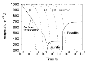
The CCT diagram gives us a critical cooling rate which we must achieve to avoid the formation of pearlite. Assuming a linear cooling rate, the CCT diagram was calculated, showing that cooling has to be faster than 0.05 K/s to avoid pearlite in alloy A. 1
To test the applicability of the calculations and to investigate the depth which can be transformed a ‘chunk’ of steel was taken of dimension 90 mm × 78 mm × 78 mm. The samples was austenitised at 1000∘C and transformed at 200∘C by transferring between two muffle furnaces. Cooling was carried out in air at room temperature, monitoring the outer surface with a probe thermocouple to ensure that it remained above 200∘C. After transformation 1 cm squared rods were cut from the block by electrical discharge machining, one through the centre of the block from the top to the bottom, and one along the base of the block. Hardness traverses were made along these rods, with several indents taken at each distance, summarised by the average and the error taken as twice the standard deviation.
To produce experimental TTT and CCT diagrams, samples were prepared from alloy A in the as–received pearlitic condition. Cylindrical samples of length 12 mm and diameter 8 mm were cut by electric discharge machining. Homogenisation was performed by sealing the samples in partially evacuated quartz tubes back-filled with argon before a heat treatment of 1200∘C for 2 days followed by furnace cooling. These samples were austenitised for 15 min and then transformed in the thermecmaster, either at different cooling rates, or at different isothermal temperatures to study the pearlite transformation. The thermecmaster is a type of dilatometer which heats the sample by induction in vacuum and it is possible to cool at selected cooling rates. Rapid quenching is possible using inert gas. The temperature is controlled by a feedback loop with a R–type (Platinum/Platinum-13%Rhodium) thermocouple welded to the sample. The dimension changes of the sample are monitored using a laser dilatometer positioned at the sample mid-length.
A number of as–cast samples were sealed in quartz tubes and austenitised and cooled in furnaces with cooling rates between 360–6∘C h−1. For the slowest cooling rate the sample was cooled to around 600∘C before removing the sample from the furnace, since transformation was expected to be complete.
Samples were bisected and examined after the experiments by standard metallographic techniques. Hardness measurements were made after diamond polishing, using a Vickers hardness testing machine with a diamond pyramid indenter.
Thermodynamic calculations were made using mtdata with the tcfe database.
A computer program cool2t3 was developed to perform the calculation of Scheil’s additivity rule, equation 3.1. This allowed calculation of CCT diagram for any cooling curve by implementing the equation for the temperature as a function of time within the program. The design allows the program to be extended in future to read an arbitrary temperature profile from a file.
For calculation of the CCT, the TTT diagram was calculated from a modified MAP_STEEL_MUCG73 program, edited to provide the transformation time with temperature resolution of 1∘C. This necessitated further changes to the program, so that the calculation of the critical temperatures were consistent with changing step size of the calculation. In the new version the critical temperatures for bainite and martensite transformation are calculated using interpolation to find the intersection of the free energy curves rather than using extrapolation based on linear regression. With other changes this resulted in the updated MAP_STEEL_MUCG83.
The linear cooling curve calculation was repeated using cool2t3 with the results from MAP_STEEL_MUCG83. The depth of material which can be hardened by bainitic transformation at 200∘C was calculated using an analytical model of heat-flow. The error–function solution for 1–dimensional heat flow in a semi–infinite surface was implemented in cool2t3. The temperature at each point and time can then be calculated assuming the surface can be instantly cooled and held constant at 200∘C, and the thermal diffusivity was taken as 1.172×10⁻⁵ m2s−1 for a steel Fe-1C wt% [164]. Figure 3.2a and 3.2b show the results, the continuous cooling curve shown is similar to figure 3.1. The calculation of the depth below the surface indicates that very large sections of material can be cooled and transformed to the bainite. It is relatively easy to avoid the diffusional products. The CCT diagrams indicate that there is a possibility of transforming to bainite at temperatures above 200∘C during cooling. If true it may be necessary in large sections to suppress the bainite start temperature if isothermal transformation of bainite is desired.
As can be seen from figures 3.3 a uniform hardness was achieved throughout the ‘chunk’. Microstructural investigation showed transformation to bainite occurred throughout from the edge to the core. The microstructure in the slowest cooling positions of the chunk can be seen in figure figures 3.4a–3.4c, since the material had not been homogenised prior to austenitisation there is a difference in etching between low–alloy and high–alloy areas but with both areas having similar microstructures.
The bainitic microstructure was achieved throughout the chunk, demonstrating the possibility of low–temperature isothermal transformation to bainite in large components without the need of any special arrangement to achieve for rapid cooling. To more quantitatively investigate the transformation kinetics of the pearlite reaction, a series of continuous cooling and isothermal transformation experiments were performed using alloy A.
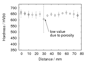
(a) Traverse through core of block, from upper surface to the base.
The low value at center and much of the scatter is caused by porosity
introduced as casting defects.
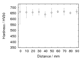
(b) Traverse across the base of the block.
Isothermal transformation experiments were also conducted to compare directly with the calculated time–temperature–transformation diagram. From these experiments it is possible to observe the start of the pearlite transformation by the expansion caused.
Figure 3.5 compares the measured isothermal pearlite transformation kinetics against the calculated transformation kinetics. The pearlite initiates sooner than expected, and at higher temperature than expected. Both may be due to over–extrapolation of the thermodynamic model used within the mucg program, or an assumption that the transformation will always begin after cooling below the α + γ/γ phase boundary without considering the eutectoid temperature caused by the α + Fe3C/γ boundary although this has not been investigated.
At temperatures from 675–700∘C the dilatation curve first contracts a little and then expands with typical S-shape Arrhenius type transformation, as shown in figure 3.6. At 500∘C the steel showed expansion but not the classic S-curve, instead expansion occurred for around 3 h and then contraction until the test was ended after 10 h as shown in figure 3.7, resulting in microstructure shown in figure 3.7b. More detailed investigation using optical microscopy to characterise multiple samples would be the best way to resolve the kinetics at these temperatures. This was not done because the major concern was the cooling past this region and that information is contained in the continuous cooling experiments, and would also be more affected by the position of the ‘nose’ of the curve in the time–temperature–transformation diagrams. Figure 3.8 shows the microstructure after transformation at 650∘C in this case the extent of pearlite transformation is greater and it is not possible to clearly distinguish any cementite on the grain boundaries.
It was also observed that a contraction was clearly evident before the onset of expansion during isothermal holding at many temperatures. The contraction initiated almost instantaneously upon cooling to the isothermal transformation temperature, perhaps even occurring during the cooling stage, such that the onset was not possible to distinguish. As shown in figure 3.9 this dilation is associated with the formation of cementite on the grain boundaries prior to the transformation to pearlite. This may be leading to faster than predicted initiation of pearlite.
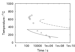
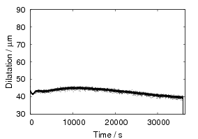
(a) Dilatation Curve
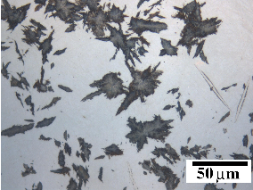
(b) Microstructure
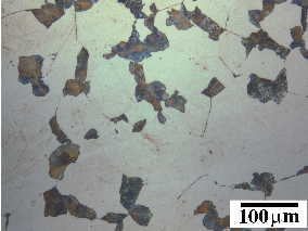
The equilibrium diagram for alloy A is shown in figure 3.10. The calculation confirms that the steel composition is pro-eutectoid, with cementite an equilibrium phase at temperatures up to 830∘C, and ferrite an equilibrium phase at temperature up to 760∘C. At austenitisation up to 980∘C vanadium carbide will be present, vanadium was purposely added to achieve this effect in an effort to limit grain growth during austenitisation.
Samples were austenitised and furnace cooled at rates between 6-360 K s−1 all transformed to fully pearlite microstructure with only the scale of the pearlite interlammelar spacing altering. The appearance of 5-10% of lighter etching areas in the microstructure also appears to be pearlite since lamellae are also visible in these regions in some cases. The microstructures can be seen in figure 3.11, and results are summarised in table 3.1. The steel transformed to pearlite when cooled at 0.1∘C s−1 which is faster than the calculated critical cooling rate which was 0.005∘C s−1 for linear cooling.
| Rate | Target Rate | Microstructure |
| ∘C h−1 | ∘C s−1 | |
| 6 | 0.0016 | Fully Pearlite |
| 36 | 0.01 | Fully Pearlite (5-10% light etching areas) |
| 72 | 0.02 | Fully Pearlite (5-10% light etching areas) |
| 360 | 0.1 | Fully Pearlite |
Further experiments were performed in the themecmaster dilatometer, and the continuous-cooling transformation diagram was produced, figure 3.12. The onset and cessation of transformation were determined by eye from the change in slope of the dilation-time curve. Figure 3.13a shows the microstructure of unhomogenised alloy A cooled at 0.16∘C s−1, and figure 3.13b homogenised alloy cooled at 0.1∘C s−1, at both these cooling rates the microstructure is largely pearlite. In these cases the lighter etching areas can be identified as martensite.
Cooling at 0.2 and 0.3∘C s−1 was fast enough to avoid pearlite as measured by the dilatation curve. As can be seen in figure 3.14 there is good agreement between the critical cooling rate to avoid pearlite as measured by cooling experiments, and the position calculated from the TTT measurements using the equation given by Scheil. The agreement between the two sets of thermecmaster experiments can be expected since it is reasonable that the detectability is similar during isothermal transformation and continuous cooling. Observation of the microstructure at faster cooling rates revealed that quantities of pearlite did form in these samples (0.3–0.7∘C s−1), figure 3.15, the minimum amount of transformation detectable by optical microscopy is smaller than that in the dilation curve.
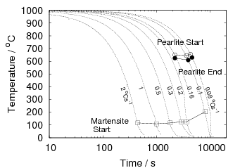
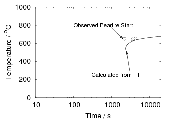
As can be seen in figure 3.16, the formation of martensite in this high carbon steel leads to the formation of micro-cracks. Although water quenching to martensite gives a harder steel than isothermal transformation at 200∘C it can be expected to be much more brittle due to the existence of so many cracks in the microstructure.
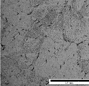
It has been demonstrated that transformation to bainite at low–temperatures can be achieved even in large chunks of material.
Methods have been implemented to allow calculation of the start time from cooling curves and the time–temperature–transformation diagram based on the Scheil additivity hypothesis. For linear cooling experiments agreement was found between the critical cooling rate determined using this method and that determined from the TTT data. These methods can allow design of steels with the appropriate transformation rate based upon the dimensions of components required.
The time–temperature–transformation calculation was found not to match the experimental results for pearlite. The pearlite in this steel being accelerated by the precipitation of cementite, which precipitates first due to the pro-eutectoid composition. The formation of pro-eutectoid cementite on austenite grain boundaries occurs quickly. It is a possibility that the cementite exists at the grain boundaries of the low–temperature bainitic steels developed to date, which can be expected to have a negative effect upon the toughness.
This chapter is concerned with the characterisation of the bainitic microstructure formed by transformation at low temperatures, principally by X–ray diffraction, optical and electron microscopy. After cooling to the transformation temperatures of 200 and 150∘C, the bainitic microstructure evolves during prolonged holding, taking many days or even months to reach completion [3]. Figure 4.1 shows the typical heat treatment profile after initial casting and forging.
Alloys were received after casting in 25 kg or 50 kg ingots and forging. These were typically reduced by around 50% by hot forging. Prior to bainite formation it is important that any heat treatments include slow cooling through the range 700-550∘C to ensure that pearlite forms because transformation to martensite would introduce microcracks.
Rods of 3 mm diameter were produced by electrical-discharge machining from alloy A, sealed in quartz tubes back–filled with argon, and homogenised for 2 days at 1200∘C. Samples were removed and re–sealed in fresh quartz tubes for austenitisation at 1000∘C for 15 min. To aid fast cooling the tubes were shattered before transfer of the rod into a second furnace where the material was transformed at 200∘C held in an alumina boat.
Hardness tests were performed on 3–4 mm lengths of the rod, mounted in Bakelite, using three hardness indents of 30 kg load with Vickers diamond pyramidal indenter.
After transformation the rods were sliced to around 250 μm discs using a silicon carbide cutting wheel, and ground to 40–100 μm using 1200 grit silicon carbide papers. These were thinned to produce samples for transmission electron microscopy using a twin jet polishing machine using a solution of 80% ethanol, 15% glycerol, and 5% perchloric acid. Polishing voltages were varied between 20 and 40 V.
Before electropolishing the samples were analysed using X–ray diffraction to measure the ferrite and austenite volume fractions and lattice–parameters. Disc samples were attached using vacuum grease in a 3×3 square onto a silicon wafer, and placed in Philips PW1730 X-ray diffractometer. Unfiltered Cu Kα radiation was generated from an X–ray tube using 45 kV and 45 mA accelerating voltage and current.
Peak positions and intensities were fitted using Philips Profit software, to find
lattice parameters and the volume fraction of austenite. Lattice parameters
were calculated using Cohen’s method [167, 168] modified to account
for the predominant errors in counter diffractometers due to specimen
displacement and specimen flatness both of which have a dependence on
peak position of the form cos 𝜃 cot 𝜃 [169, 170]. The phase fractions were
calculated using the method proposed by Dickson [171, 172]. This method
calculates the phase fraction  by weighting the contribution of each peak
measured by the inverse of the expected intensity of the peak Iγ(hkl) and
Iα(hkl).
by weighting the contribution of each peak
measured by the inverse of the expected intensity of the peak Iγ(hkl) and
Iα(hkl).
![Iγ(hkl) Rγ(hkl)[ X γ]
------ = ------- ---
Iα(hkl) R α(hkl) X α](superbainite135x.png) | (4.1) |
where R for each peak is calculated from the volume of the unit cell v, structure factor F, multiplicity factor p, temperature factor e−2m and L P the Lorentz-polarisation factor.
![1 [ ]
R = ---|F |2(p)(LP ) e−2m.
v2](superbainite136x.png) | (4.2) |
These calculations were performed using a modified version of the program MAP_CRYSTAL_XRDCALC [173], version 1.2 [174].
Rietveld analysis [175, 176], fitting the whole diffraction pattern at once, was also applied to the data using Philips Highscore–plus software. This second technique also allows extraction of phase–fractions and lattice parameters.
Once lattice parameter values were obtained, carbon content of ferrite and austenite were then calculated using relations proposed by Dyson and Holmes [177, 178];
where aγ is the lattice parameter of austenite in Ångstroms, and Wi is the concentration of element i in weight percent. where aα is the lattice parameter of ferrite in Ångstoms, and xi is the concentration of element i in mole fraction.A martensitic sample was produced by shattering the quartz tube during quenching into water from the austenitisation temperature of 1000∘C (after 15 min holding as before). Data for the martensite were analysed to test the method, since austenite and ferrite can both be expected to inherit the bulk composition. Correct analysis of martensite lattice parameters is only possible when the extra peaks due to tetragonality of the martensite lattice can be resolved. The equation for carbon content was applied by taking the cube–root of the volume of the unit cell. The carbon contents calculated in this way had good agreement with the carbon contents expected in the martensite.
Transmission electron microscopy utilised JEOL 200 CX (TEM), high resolution scanning electron microscopy was conducted on JEOL 6340F which has cold–tip field emission gun (FEGSEM). Lower resolution scanning electron microscopy such as examination of fracture surfaces utilised JEOL 5800 with energy–dispersive X–ray spectrometer (SEM).
To determine the bainite plate size, measurements were made on transmission and scanning electron micrographs. The mean linear intercept in the direction normal to the plate length, T is related to the average true thickness by T = πt∕2.
For alloy A transformed at 200∘C a total of 481 plates, 60% of the measurements were made on transmission electron TEM micrographs after transformation for 7 days. The remaining measurements were made after 10 days of transformation, using both FEGSEM and TEM micrographs. There was little difference between the 3 data sets so they were combined and presented as a single distribution.
Tensile samples of alloy A were also transformed at 200∘C for 12 days and 150∘C for 2 months, after austenitisation at 1000∘C for 15 min sealed in quartz silica tubes, using same procedure as before for transfer between furnaces.
Tensile samples of Alloy C were transformed at 150∘C for 1 year. Following mechanical testing, thin sheets of material were sectioned using a silicon carbide cutting wheel from the head of the tensile sample and 3 mm discs were punched and then prepared for TEM using the methods previously described.
The hardness was found to be 643 ± 11 HV30 in the material transformed for 10 days at 200∘C, decreasing to 626 ± 9 after 1 h tempering at 400∘C. As can be seen in table 4.1 the hardness is similar after 10, 11 and 12 days. The hardness of martensite formed on water quenching is higher, but reduces to a greater extent upon tempering for the same time.
| Alloy & Condition | Transformed hardness HV30 ±2σ | Tempered hardness HV30 ±2σ |
| Alloy A; |
|
|
| - Water Quenched | 721±18 | 606±20 |
| - 10 days at 200∘C | 643±11 | 626±9 |
| - 10 days at 200∘C (2) | 646±12 | 621±14 |
| - 11 days at 200∘C | 636±10 | 624±16 |
| - 12 days at 200∘C | 643±14 | 617±22 |
| - 2 months at 150∘C | 617±19 | 555±20 |
| Alloy C |
|
|
| - 1 year at 150∘C | 635±6 | 602±10 |
Figure 4.2 shows the optical microstructure after transformation for 12 days at 200∘C. On this scale it is only possible to see the coarse structure of the bainite sheaves. Higher magnification microscopy is necessary for resolving the individual plates and thin–film austenite as shown in the scanning and transmission electron images, figures 4.3–4.7. The indexing of the X–ray diffraction pattern, figure 4.8a, confirms the presence of residual austenite, as expected from the previous work discussed in Chapter 1. Results of peak profile fitting and Rietveld refinement to determine phase fractions and lattice parameters are summarised in table 4.2. The lattice parameters for austenite and ferrite were converted to carbon contents suggesting that both phases are supersaturated with carbon. Figure 4.9 shows the measured carbon contents and compares austenite content to the thermodynamic limit given by T0. The carbon content in the austenite is at the level predicted by this thermodynamic limit. The figure uses the results of the Rietveld analysis which gave more robust results than the peak fitting, although the results were generally in agreement using the two techniques.
The results determined by analysis of X-ray diffraction patterns are very similar for transformation after 10 and 12 days, as were the hardness values. This is because transformation asymptotically approaches completion and is essentially complete after 10 days, with little change expected with prolonged holding. It should be noted that the values determined for phase fraction and carbon contents account for 0.7 wt% carbon, whereas the bulk carbon content is 0.79 wt%. The carbon contents were further investigated using atom–probe tomography the results of which are presented in a later chapter. To identify any carbides in the steel after transformation for 200∘C for 10 days, the matrix was dissolved using 5% nital solution for several days, followed by filtration using 0.2 μm polycarbonate film. The residual material was then analysed by X-ray diffractometer, the pattern in figure 4.8b, matches a face-centred cubic (FCC) unit cell with lattice parameter around 4.1 Å, corresponding to vanadium carbide, but could also match aluminium used in the sample holder which can be illuminated by the X-rays at low angles. The peak positions match either phase, but the relative intensities of the first two peaks best match aluminium, so that vanadium carbide is not positively identified from this scan. It is possible that there is also an amount of epsilon-carbide present which would explain the small peaks present at 41 and 57 ∘2𝜃 with other expected peaks overlapping with the FCC phase. Small cementite particles (approximately 20 nm wide 175 nm in length) were previously observed in this steel by Caballero et al. [3] after transformation for 2 weeks at 190∘C as mentioned in Chapter 1.
The carbon contents determined from the lattice parameters did provide a good agreement with the expected carbon content in the sample water quenched to form martensite. The fitting of the X–ray diffraction pattern for the martensite necessitated allowing for tetragonality, which was only possible in this case using the full pattern fitting of the Rietveld analysis. Carbon content was determined to be 0.74 wt% in austenite and 0.79 wt% in the martensite. The error bars determined using Rietveld refinement were calculated from the deviation of the relevant parameter which is determined during the fitting (in this case lattice parameter) and seem to underestimate the error especially compared to the values determined from the peak fitting where the error was estimated from the variance of the lattice parameters determined using each indexed peak.
The retention of high carbon austenite is thought to be desirable for mechanical properties, since it can lead to increased toughness by transformation–induced plasticity. However, large areas of retained austenite ‘blocks’ must be avoided since they are likely to cause crack initiation by formation of brittle martensite. As can be seen in figure 4.3(a,b) the large fraction of ferrite achieved leads to micron-scale austenite blocks.
The results of plate size measurements on alloy A are shown in table 4.3 after stereological correction, showing that the average plate thickness is between 34 and 41 nm. Taking the whole of the data the average plate thickness was taken to be 39±1 nm, this was the same value if taking all of the data from TEM and, FEGSEM measurement after transformation for 12 days, or the data as a whole (also table 4.3). The error of the mean value was estimated by considering the standard error, this value would be the same as the standard deviation if the plate size measurements were uniform, however a large distribution in apparent plate sizes was recorded. One reason for this is the bisection of the plates at various angles to their thickness, but it also possible that there is a real distribution in the plate thicknesses. As shown in figure 4.10 a large distribution is seen in the plate size measurements. The TEM micrographs in figures 4.6 and 4.7, show areas of parallel plates of similar thicknesses. These can be expected to have been bisected at the same angle. In some cases it is difficult to resolve the plate size, which may lead to a broader distribution in the measurements and there is also the possibility that adjacent plates may merge (recoalescense). As shown in figure 4.5 in some areas smaller platelets are difficult to distinguish from larger plates. Due to nucleation of plates along side existing plates, these features can be seen as parallel striations at a constant angle along the length of a plate, or as individual plates (platelets or sub-units) inside a larger sheaf. How they are regarded will depend upon the resolution of the technique used, and the particular arrangement observed.
Figure 4.10(b) compares the observed distribution of plate widths against that expected if semi–infinite plates are bisected at random angles (line A - cos 𝜃), as can be seen that would result in a much sharper distribution. Therefore there should be other contributions to the observed widths, such as variation in the thickness of the plates, or effect of thin–foil specimen. Line B compares the distribution against cos 𝜃 cos ϕ.
Some evidence of carbide precipitation was observed, for example in figure 4.4(b) shows nanometre scale round particles, presumably carbides, on the ferrite–austenite interfaces.
Further reducing the transformation temperature from 200 to 150∘C did not lead to any measurable carbon enrichment in the austenite. Neither of alloys transformed at 150∘C exhibited any measurable carbon enrichment in the austenite above the bulk carbon content. Compared to the result of transforming at 200∘C a slightly larger fraction of ferrite is measured in the samples transformed at the lower temperatures, and the carbon super-saturation in the ferrite is also greater. This measurement is supported by the greater reduction in hardness upon tempering for 1 h at 400∘C when compared to the bainite formed at 200∘C. Despite the different compositions and holding times the results are similar for both the samples transformed at 150∘C. Increased trapping of carbon at dislocations as temperature is lowered is one possibility, but dislocation density resulting from martensitic transformations is expected to be constant below 300∘C [21]. Undetected carbide precipitates are a possibility due to the missing balance of carbon when considering ferrite and austenite lattice parameters. Inhomogeneity of carbon content in the austenite could be a possible explanation. For example if carbon is trapped in the thin films austenite which produces very broad peaks, the lattice parameter determination could still be dominated more by position of the remaining bulk austenite peaks 1 .
TEM micrographs of alloys A and C transformed at 150∘C can be seen in figures 4.11–4.16. In comparison to the width of plates after transformation at 200∘C the plate size was larger again at the lower temperature, accompanied by a larger spread of plate size measurements, as seen in the larger standard deviation shown in table 4.4 around 50 nm compared to 30 nm at the higher temperature. TEM micrographs Alloy A exhibits both very thin plates as seen in figure 4.12b, and very wide plates as shown in figure 4.14b were the feature of around 0.8 μm seems to be made of smaller sub-units of width 0.2 μm. Large and thin plates can be seen in the same areas, for example in figure 4.11a. Of course some of the difference may be due to sectioning effects as discussed earlier.
In alloy C large plates of tempered martensite were observed in the transmission electron micrographs along with the bainitic microstructure. These could easily be identified by the different morphology and excluded from the plate size measurements. It seems most likely that a small amount of martensite formed before the bainite transformation and subsequently tempered during the prolonged holding time at 150∘C, despite the temperature of isothermal transformation being above that for martensite start measured using dilatometer of 120∘C [103].
The lack of significant carbon enrichment leaves the possibility of a small amount of martensite forming upon cooling to room temperature after isothermal transformation at 150∘C. Despite this, large areas of retained austenite were observed in alloy A in the TEM micrographs. Transformation time for alloy A was estimated based on previous experimental results for the same alloy [3] to give a microstructure with majority of bainite. Alloy C transformation time was increased to 1 year to ensure the maximum amount of transformation. Despite this, some features could be identified likely to be martensite due to the presence of a mid–ridge and the angle between adjacent plates. However, in alloy C the volume of martensite formed during cooling should be very small.
Stress–strain curves for tensile testing after transformation at 200 and 150∘C are shown in figure 4.17. Transformation of alloy A resulted in an average tensile strength of 1.2 GPa, the total elongation is very low, below 1%, so that 0.2% yield strength could not be determined. Previous work tested this alloy in compression and determined the yield strength as 1.96 GPa. So it seems that the alloy is too hard, that there are too many barriers to dislocation movement, so that any imperfections cannot be tolerated and cause ‘premature’ failure.
When transformed at 150∘C the tensile strength dropped to around 600 MPa UTS, 450 MPa yield strength, still with total elongation around 1%. Alloy C transformed at 150∘C resulted in ultimate strength of 1.4 GPa, yield strength of 970 MPa and elongation around 2%. This compares with an ultimate tensile strength of 2.15 GPa UTS and yield of 1.4 GPa and elongation of 5% in the same alloy transformed at 200∘C (table 1.7).
Fractographs of typical samples of A transformed at 200 and 150∘C can be seen in figures 4.18 (a) and (b). The initiation point of each failure is around 100 μm below the outer surface of the tensile piece, having a faceted appearance, but the fracture surface shows more ductility away from the initiation point. It was not possible to locate any defect responsible for fracture initiation using energy dispersive spectroscopy, back scattered and secondary electron imaging in the SEM. Cross–section analysis through the initiation point, figure 4.19, shows that fracture initially propagated by crack growth along the prior austenite grain boundaries, leading to the faceted appearance.
The lower yield strength of alloy A and C after transformation at 150∘C is consistent with the lower carbon content, possibly due to the lower strength of the austenite. Lower UTS and elongation can also result if austenite can too easily transform to brittle martensite, or martensite can transform at too high a rate reducing the beneficial effect of that the TRIP effect could have on the elongation.
| Alloy, condition | Austenite | |||
| Volume /% | Lattice Param. /Å | Carbon /wt% | ||
A, 200∘C 10 days. | P | 35.4 ±0.08 | 3.6185 ±0.003 | 1.11 ±0.2 |
| R | 21.5 ±1 | 3.6235 ±0.002 | 1.27 ±0.1 | |
A, 200∘C 12 days | P | 21.3 ±0.07 | 3.6209 ±0.01 | 1.19 ±0.3 |
| R | 20.5 ±3 | 3.6239 ±0.002 | 1.28 ±0.1 | |
C, 150∘C 1 year | P | 21.6 ±0.05 | 3.6071 ±0.004 | 0.77 ±0.1 |
| R | 20.4 ±0.4 | 3.6083 ±0.0003 | 0.80 ±0.1 | |
A, 150∘C 2 months | P | 18.9 ±0.09 | 3.6016 ±0.003 | 0.60 ±0.1 |
| R | 17.1 ±0.11 | 3.6067 ±0.0004 | 0.76 ±0.01 | |
A, quenched | P | 27.5 ±0.02 | 3.6106 ±0.005 | 0.87 ±0.15 |
| R | 14.2 ±0.4 | 3.6063 ±0.0002 | 0.74 ±0.01 | |
| Alloy, condition | Ferrite | |||
| Volume /% | Lattice Param. /Å | Carbon /wt% | ||
A, 200∘C 10 days. | P | 64.6 ±0.08 | 2.8759 ±0.002 | 0.27 ±0.06 |
| R | 78.5 ±1.2 | 2.8772 ±0.001 | 0.31 ±0.03 | |
A, 200∘C 12 days | P | 78.6 ±0.07 | 2.8738 ±0.005 | 0.20 ±0.17 |
| R | 79.5 ±3 | 2.8759 ±0.001 | 0.27 ±0.03 | |
C, 150∘C 1 year | P | 78.4 ±0.05 | 2.8758 ±0.002 | 0.26 ±0.06 |
| R | 79.6 ±0.4 | 2.8774 ±0.0003 | 0.32 ±0.01 | |
A, 150∘C 2 months | P | 81.8 ±0.1 | 2.8704 ±0.0005 | 0.08 ±0.02 |
| R | 82.9 ±1.7 | 2.8818 ±0.0003 | 0.47 ±0.01 | |
A, quenched | P | 72.5±0.02 | 2.9308±0.04 | 2.17±1.4 |
R |
85.8±0.4 | 2.8679±0.0002 |
0.79 ± 0.01 |
|
| 2.9380±0.0003 | ||||
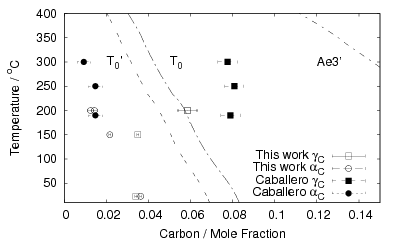
(a) Alloy A at 200 and 150∘C isothermal transformation, and martensite formed by water
quenching to room temperature, previous result for this alloy added from Caballero et al. [3].
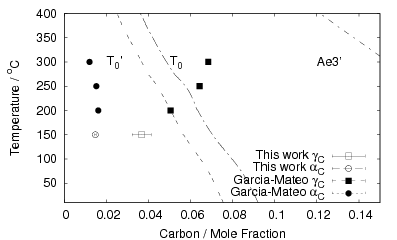
(b) Alloy C transformed at 150∘C, previous results added from Garcia–Mateo et al. [4, 105].
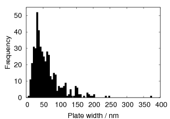
(a) Plate widths
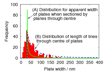
(b) Comparison against possible stereological distributions.
Condition | 7 days TEM | 12 days TEM | 12 days FEGSEM |
Mean width | 41±2 nm | 34±2 nm | 39±3 nm |
Standard deviation | 29 nm | 23 nm | 26 nm |
Median width | 34 nm | 27 nm | 31 nm |
Number of measurements | 283 | 102 | 94 |
 ).
).
Alloy & | A 200∘C | A 150∘C | C 150∘C |
Condition | 7 & 12 days | 2 months | 1 year |
Mean width | 39 ±1 nm | 63 ±4 nm | 51 ±4 nm |
Standard deviation | 27 nm | 49 nm | 58 nm |
Median width | 31 nm | 53 nm | 51 |
Number of measurements | 479 | 127 | 78 |
).
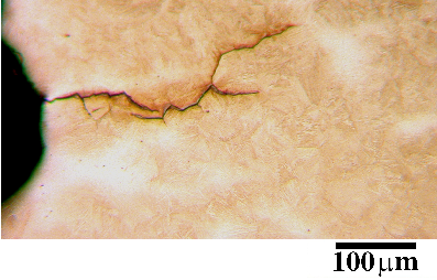
Alloy A has been transformed into fully bainitic condition at 200∘C and this material is used to research different tempering heat treatments, as presented in a later chapter. The bainite forms with high carbon supersaturation in ferrite and austenite, with carbon in austenite at the level predicted by T0.
The fine bainite plate size being the most dominant strengthening mechanism in these steels, many measurements were made for alloy A transformed at 200∘C, determining the plate width to be 39±1 nm. This size is at the upper end of the range observed in previous studies of 20-40 nm.
Contrary to the trend expected from extrapolation of higher temperature results, the plate width is found to become larger again when reducing the temperature to 150∘C in both Alloys A and C. This suggests that there may be an optimum temperature for achieving the smallest plate size. The increase was accompanied by an increase in the spread of plate sizes as measured by the standard deviation suggesting coalescence of plates may be an explanation. The possibility of some martensite transformation, and the question of distinguishing carbide free bainite from isothermally transforming martensite could cause some difficulty to interpreting the results.
Transformation at 150∘C was also interesting in that no carbon enrichment was measured in the austenite either in alloy A which can be expected to be near the end of bainitic transformation, or in alloy C which had more than ample time to transform.
Transformation at low–temperatures can result in a very hard microstructure, in the tensile samples tested failure occurred abruptly from grain boundaries and at lower strains than have been previously reported in other similar steels. High strength steels can be expected to be less tolerant to any defects, especially when the yield strength is high.
In this chapter the structure achieved by isothermal transformation at 200∘C is characterised using atom probe microscopy. As described in Chapter 1, low temperature transformation of bainite is achieved by the use of a high average carbon concentration and to some extent, substitutional solutes such as manganese. The silicon concentration is such that a precipitation of carbides from austenite is prevented during the bainite reaction. The microstructure following isothermal transformation is quite simple, a mixture of bainitic ferrite and carbon–enriched retained austenite. The austenite occurs either as films between the ferrite plates or as fine blocks bounded by bainitic sheaves.
X–ray diffraction analysis of the retained austenite has shown that it is enriched in carbon to a concentration close to the T0 boundary, as expected from the incomplete reaction phenomenon. The T0 boundary on a temperature versus carbon concentration plot is the locus of points at which the Gibbs free energies of austenite and ferrite of identical composition are equal. The X–ray analysis also revealed a considerable supersaturation of carbon in the bainitic ferrite. Similar supersaturation has been measured previously using atom probe analysis [50, 51, 52] and convergent beam electron diffraction analysis [179] in low–carbon steels. This supersaturation was attributed to the trapping of carbon at the dislocations in the bainitic ferrite [21].
The previous compositional studies of the new high–carbon bainite of interest have been performed using X–ray lattice parameter measurements. They represent coarse measurements whereas the scale of the structure is very fine. It was therefore decided to use atom probe tomography to obtain more detailed information, particularly of the fine scale distribution of carbon. The tomographic atom probe used has the ability to collect large quantities of atomic data, which can then be compared against theory.
Atom probe techniques were originally developed by E. W. Müller, as an extension of the field emission microscope which he introduced in 1935 [180]. The high field strength required for electron emission from a solid by quantum tunnelling [181, 182] was achieved by shaping the specimen into a sharp tip. Müller found that by reversing the bias of the emitter and introducing a small amount of a pure gas, cations could be used to form a magnified image of the specimen [183]; this technique is used in the ‘field ion microscope’, figure 5.1a. On October 11th 1955 Kenwar Bahadur and Prof. Erwin. W. Müller first succeeded in using the field ion microscope to image individual tungsten atoms, using liquid nitrogen to cool the specimen and helium as an imaging gas. Prof. Müller proclaimed ‘Atoms, ja, atoms!’[184].
It was discovered that raising the potential above that needed for imaging with gas caused atoms to evaporate from the surface. This allowed preparation of clean samples, and was an important factor allowing Bahudur and Müller to image individual atoms. ‘Field evaporation’ later led to tomographic and mass resolution techniques.
Müller further extended the design of the field ion microscopes to incorporate mass resolution [185], by using a pulsed voltage which allowed time of flight mass spectrometry of atoms evaporated from the sample tip. The first such microscope was developed by Müller, Panitz and McLane in 1967 [185]. Further improvements where made by Panitz in the 1970’s with the ‘imaging atom probe’ [186]; using a time-gating mode the distribution of a single element on the sample surface could be mapped.
Inspired by Panitz’s work, Miller developed the concept of the three dimensional (tomographic) atom probe, figure 5.1b, implementing the first prototype in 1986 [187]. The light signal generated by an ion hitting a phosphor screen is split into two channels, one using a charge–coupled device (CCD) to detect the position, and the other signal going to an array of photo–diodes to determine the time of flight. The first fully operational unit for three dimensional imaging was the position–sensitive atom probe (PoSAP) developed by Cerezo et al. [188] in 1988. A variety of designs have been developed including detectors based on CCD or video cameras and multi–anode arrays.
Kelly et al. [189] developed a local electrode atom probe (LEAP) which allows greater concentration of the field strength around the tip by bringing it into close proximity to a counter electrode as first suggested by Nishikawa and Kimoto [190]. This allows greater mass resolution and increased field of view, data acquisition time has also been increased by improved instrumentation.
The composition of the steel is given in table 5.1. Samples were prepared from a billet of 25 kg. After casting the ingot was cooled to ambient temperature, then hot rolled into plate 40 mm thick and 75 mm wide. Sections of approximately 40 mm × 40 mm × 75 mm were machined, and then homogenised for 48 h at 1200∘C. Care was taken to avoid martensite formation by slowly cooling the sample after each heat treatment. Rods 3 mm in diameter were then made by electrical spark erosion and sealed in quartz tubes with an argon atmosphere at 0.9 bar. They were then austenitised by placing in an oven preheated to 500∘C followed by continuous heating to 1000∘C where they were held at that temperature for 15 min. After austenitisation, the rods were removed from the quartz tubes and allowed to cool to the isothermal transformation temperature of 200∘C and were held at that temperature for 12 days. The heat treatment is based on the measured TTT diagram and results from a similar composition alloy (alloy A) [3]. Atom probe tomography characterisations were performed in the ORNL energy–compensated optical position–sensitive atom probe (ECOPoSAP). The experiments were performed at a specimen temperature of 60 K, a pulse repetition rate of 1.5 kHz, and a pulse fraction of 0.2 of the standing voltage.
Using the position–sensitive atom probe it is possible to analyse a volume which has an area of around 10–20 nm squared with a depth up to 250 nm, such an area contains around 1 million atoms.
Alloy | C | Si | Mn | Ni | Cr | Mo | V | Al | P | S | Units |
E | 0.75 | 1.63 | 1.95 | 0.0 | 1.48 | 0.28 | 0.1 | 0.01 | 0.003 | 0.003 | wt% |
E | 3.34 | 3.10 | 1.90 | 0.0 | 1.52 | 0.16 | 0.1 | 0.02 | 0.005 | 0.005 | at.% |
The standard method of preparing metal samples for atom probe analysis uses two or three stages of electro–polishing. In the first stage the sample is suspended in a thin layer of electrolyte, which floats above a dense layer of inert liquid, as shown in figure 5.2a. In this way the middle section of the sample can be selectively etched and thinned. Through all stages of etching it is necessary to observe the sample using a binocular microscope to allow control the etching process. The sample is raised and lowered to prevent preferential etching at the air–electrolyte interface, and enable selective polishing to improve the taper angle of the tips. The electro–polishing conditions are chosen to allow material to be eroded rapidly and reasonably uniformly. Stage one electro–polishing is stopped just before separation of the two halves. Further thinning is more controlled to allow more uniform polishing, a less aggressive electrolyte is substituted, and since the sample is already tapered from stage one, it is no longer necessary to use an inert layer. The sample is lowered into the electrolyte, the thinning is monitored with a microscope, stopping the current when the sample separates into two halves.
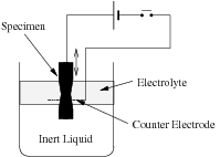
(a) Stage one
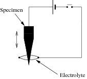
(b) Stage three, ‘drop–polishing’
Observation with a good optical microscope is used to access the two tips produced, a good sample having a sharp taper angle near the tip and an even polish. Further etching to sharpen the tip using the ‘dip’ or ‘micro–polishing’ method shown in figure 5.2b is usually necessary for the bottom half of the sample which falls into the electrolyte. In the ‘drop–polishing’ method a drop of electrolyte suspended in a wire loop. The sample is raised and lowered with the tip moving through the lower surface of the drop. The current is pulsed, switching off just before the end of the tip moves into the drop. As material is removed from the tip it may be necessary to change the electrolyte, if the tip is close to being sharp enough then care must be taken not to lower the tip through the top surface as the surface tension is enough to bend the tip.
Stage one electro–polishing of the bainitic steel was carried out using an electrolyte solution of 25% perchloric acid and 75% acetic acid (ethanoic acid) with electrical potential of 20 volts. The electrolyte was floated on ‘Galden’ perfluoropolyether. In stages one and two a platinum counter electrode was used in the form of a wire which looped around the sample. Stage two electropolishing and the final dip polishing used 2% perchloric acid and 98% butycellosolve with the potential decreased by 2 volts, the same platinum counter electrode was used as for stage one.
Before polishing, between stages, and afterwards methanol was used to clean the sample and equipment, to prevent contamination of the sample which can cause difficulty in achieving the necessary vacuum. After etching the sharpened sample was placed in a copper stub, loaded into a nickel stub, and immediately placed under vacuum in the holding chamber of the atom probe. The stub components and sample tips are handled only with tweezers and tongs.
Field ion microscopy is almost always the start of any atom probe experiment to collect tomographic data. Some field evaporation of the tip is necessary to form an atomically sharp and clean tip and at the same time the tip is examined and some microstructural characterisation can take place before positioning the area from which tomographic data will be collected.
The sample is transferred from the holding chamber to the analysis chamber, and cooled to 20–60 K depending on the specimen material and the imaging gas. Once the temperature has stabilised and a vacuum of 2×10⁻¹⁰ mbar has been achieved in the analysis chamber a small quantity of imaging gas is admitted to a pressure of 1–5×10⁻⁵ mbar.
The standing voltage is increased until the field ion image is visible on the phosphor screen. The required potential depends on the tip radius of curvature and the imaging gas. Contamination and artifacts from sample preparation can be removed by carefully increasing the voltage until a clean and fully developed apex region is formed. Minimising the potential lowers the stress and elastic dilation in the apex region, which is of the order of 1–2% and has even been observed to cause phase transformations [191]. As shown in figure 5.3 the analysis volume is only a portion of the tip.
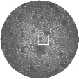
(a) Area of analysis imposed on
field ionisation microscope image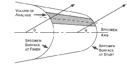
(b) Location of the volume of analysis
For each ion detected in the tomographic atom probe the time of flight to the detector and the x and y coordinates of its impact position on the two dimensional position–sensitive detector are recorded. Each ion is later identified using its mass to charge ratio and the position in the analysis volume is determined using a reconstruction algorithm, xi and yi are used to estimate the atom coordinates in the specimen, X and Y , X = xi∕η and Y = yi∕η.
The z position is determined from the order in which the ions strike the single atom detector, the position of the ion in the z direction is incremented by an amount zi for each ion impacting the detector square. Zi = ωi∕ζAd where ωi is the atomic volume of the ith ion in the phase under analysis, Ad is the effective area and ζ is the detection efficiency of the single atom detector.
This basic method is used to reconstruct the atom positions in the position sensitive atom probe. In the local electrode atom probe extra corrections need to be made due to the large field of view so the end shape of the specimen has to be taken into account.
Since not all atoms are collected or unambiguously identified, the topographic
data set is actually a sample of the atoms in a volume. The error in the
measurement can be calculated assuming a normal distribution in the error
 where ns is the number of atoms of species s and N is the total number of
atoms in the volume [184].
where ns is the number of atoms of species s and N is the total number of
atoms in the volume [184].
Figure 5.4 shows a typical atom probe result showing high carbon and low carbon regions, and the composition profile from a selected volume across the interface. Figure 5.5 shows projections of the sample volume showing the position of the various elements.
A much larger volume was obtained in one experiment as shown in figure 5.6a. The atom map shows a projection of the carbon atom positions in three dimensions obtained from a large data set. The corresponding concentration profiles from slices of equal depth along the length of the sample volume of 16 nm × 16 nm × 340 nm are shown in figure 5.7 and 5.8. Atoms are recorded from a cone–shaped volume, so the cross–section increases along the length, in this case around 5 nm × 5 nm at the tip. The error bars for each concentration point are calculated based on the procedures given above, based on the number of atoms and the total atoms in each slice. The measurements show alternating carbon–enriched and carbon–depleted regions. There are variations in the degree of enrichment. It is important to note that the carbon fluctuations in the austenite and ferrite do not correlate with substitutional solute concentrations. The measured fluctuations of chromium, silicon and manganese when represented as concentrations are within the measurement uncertainties 1 and consistent with the substitutional lattice being configurationally frozen during transformation [1]. These results are also shown in figure 5.7 and 5.8, but using ratio of number of atoms of substitutional elements against number of solvent iron atoms, since this ratio remains constant for displacive transformation. In contrast additional carbon will proportionally reduce the percentage of each element, addition of 10 at.% carbon to a region will reduce atomic fraction of each element by 10%. As can be seen in composition profiles, the ratio of substitutional elements to iron is not correlated with changing carbon contents, in fact it fluctuates about the mean value.
As the atom probe analyses generally do not give crystallographic information, carbon enrichment beyond the average value of 3.3 at.% is assumed to represent a region of austenite. This indicates the presence of austenite phases at the marked distances. Figure 5.6b–5.6d shows isoconcentration surfaces for 1, 2 and 3 at.%, the 3 at.% isoconcentration surface can also be used to distinguish the austenite and ferrite regions. The morphology of these ferrite and austenite regions can be compared to electron microscope images as shown in figures 4.4–4.7. The scale of the concentration variations matches that of the bainitic ferrite plates and austenite films.
The enrichment of austenite (> 8 at.%) with carbon is expected when some of the excess carbon partitions from the bainitic ferrite following transformation [21]. The maximum enrichment of carbon in austenite at 73 nm distance was found to increase to a maximum of 12 at.% on making the selected volume perpendicular to the austenite–ferrite interface. Similar level of carbon supersaturation has previously been achieved by gas–phase carburisation at 470∘C in 316 austenitic stainless steel and termed colossal supersaturation. The data from the ferrite regions also show carbon enrichment that is in agreement with previous X–ray studies [3, 92, 101, 103]. The presence of excess carbon in the ferrite is a consequence of the displacive mode of transformation, and the retention within the ferrite is thought to be associated with the stability of carbon within defects in the ferrite [21]. These defects trap the carbon atoms as originally proposed by Kalish and Cohen [192]. The trapping prevents the carbon from partitioning into austenite and from precipitating within the ferrite. There are detailed variations in the carbon within the ferrite, for example at 100 to 150 nm (figure 5.7 and 5.8). These are not further explained by taking the cross–section along the length of the sampled volume, or by taking cross–sections perpendicular to the major axis of the plates as shown in figures 5.9a–5.9e. Taking cross–sections through the plates confirmed similar levels of carbon for the austenite at 70 and 220 nm along the sample length (labelled A and D), but revealed extra detail at around 185 nm showing two austenite thin films both with around 4 at.% of carbon.
Field ion micrographs were acquired at the end of the experiment for the large data set (figure 5.6a), as shown in figures 5.10 and 5.11. Since the material does not share a single crystal structure, is not easy to interpret or extract crystallographic information. The surface structure is quite complex and appears quite disorderly. The tomographic data are from a region near the center of the tip as shown in figure 5.1a. It is possible that the brighter ‘finger–like’ features in the left of the figures traverse an region of parallel ferrite plates and austenite thin films, the curved appearance being caused by the tip geometry. Brighter regions may be caused by differences in chemistry and surface topography of the tip as a result of field evaporation.
Another example from a smaller data set sampling austenite and ferrite is shown in figure 5.12a and 5.12b. As in figure 5.6a, this atom map is the projected image of the three–dimensional position of carbon atoms. Figure 5.12a shows the concentration profile across the austenite and ferrite phases, with a sampling volume (indicated in the atom image in figure 5.12b) approximately perpendicular to the austenite–ferrite interface. These data show that the average carbon concentration variation across the interface is not sharp. Similar to the results in figure 5.7 and 5.8, there is no correlation between austenite and ferrite carbon concentrations to any substitutional solute concentration. There is no partitioning of substitutional elements during the bainite transformation.
The measured data are compared with paraequilibrium phase diagram calculated for the steel (table 5.1). The calculated and measured ferrite and austenite compositions are compared in figure 5.13(a). The calculated paraequilibrium concentration in ferrite is so low that it overlaps with the ordinate for the scales as illustrated. The calculations show that there is excess carbon in the ferrite, well beyond the 0.05 at.% expected from paraequilibrium at austenite at 200∘C. The average austenite carbon concentration is also somewhat higher than that of the expected T0 limit. To evaluate the sensitivity of thermodynamic information and T0 point at 200∘C, further calculations were performed using ThermoCalc software [193] with the Thermo-Tech iron database [194]. These calculations also show [see figure 5.13(b)] that the austenite carbon concentration is higher than the predicted T0 concentration. To provide a further perspective of these comparisons, histograms of measured carbon concentrations from figures 5.6a and 5.12b are shown in figure 5.13(c). To allow comparison between the two regions the data have been normalised, the area of figure 5.6a contains 2.9 million and 5.12b contains 600 000 atoms. The data show that the measured austenite carbon concentrations vary over a wide range. Earlier X–ray diffraction studies of the austenite composition showed good agreement with T0 at 200∘C [21, 51]. These are average results whereas, the atom probe results has a much higher spatial resolution. Nevertheless, the lower limit of austenite carbon concentration measured in atom probe is closer to the T0 curve, which may be considered as agreement with theoretical models for bainite transformation. The reasons why the concentration may be somewhat in excess of T0 have been discussed previously [21, 51]. Carbon can continue to partition into isolated regions of austenite although transformation to bainite cannot occur once the concentration reaches that given by the T0 curve.
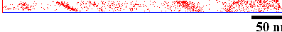
(a) Projection of tomographic element map for carbon

(b) 1 at.% carbon isoconcentration surface

(c) 2 at.% carbon isoconcentration surface

(d) 3 at.% carbon isoconcentration surface
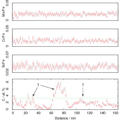
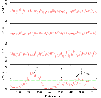
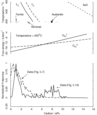
| Element | χ2 | Degrees of freedom | 0.01% of χ2 | Result | |||
| C | 33300 | 8 | 20.090 | Reject | |||
| Si | 29.4 | 10 | 23.209 | Reject | |||
| Mn | 362 | 7 | 18.475 | Reject | |||
| Cr | 27.8 | 6 | 16.812 | Reject | |||
| Mo | 15.1 | 3 | 11.345 | Reject | |||
An energy compensated optical position sensitive atom probe was used to analyse the nanoscale distribution of carbon and other substitutional solutes in a low temperature bainitic microstructure consisting of a mixture of bainitic ferrite plates in a retained austenite matrix. Atom probe microanalysis showed a wide distribution of carbon concentrations in both ferrite and austenite. The measured average carbon concentration in the austenite was 8.0±1.6 at.% and the maximum concentration was 12.0±1.3 at.%. The measured average carbon concentration in bainitic ferrite was 1.1±0.7 at.%. In ferrite regions close to the austenite, the maximum ferrite concentration was 1.8±0.4 at.%. The ferrite carbon concentrations are higher than expected paraequilibrium solubility levels. The results are consistent with previous atom–probe data on low carbon steels and confirm the supersaturation observed by X–ray analysis, as presented in detail in the previous chapter, which indicated that excess carbon persists in bainitic ferrite.
The results are fully consistent with the displacive nature of the bainite transformation, strong evidence is observed in the uniformity of substitutional elements in the ferrite and austenite.
The tempering behaviour of alloys A and B after transformation at 200∘C has been investigated using hardness testing, X–ray diffraction and transmission electron microscopy. Results for alloy B are presented in greater detail in a previous publication with Garcia–Mateo et al. [2], where TEM micrographs of that alloy in a tempered state can also be seen.
As discussed in Chapter 1, transformation at low–temperatures in these steels leads to strengthening by very thin bainite plates (20–40 nm thickness). Formation of relatively large embrittling carbides during transformation is avoided by the judicious use of silicon as an alloying element.
The hardness of low temperature bainite can be as high as 700 HV30, exceeding that of the vast majority of as–quenched martensitic microstructures. It has been suggested that the hardness of martensite becomes independent of carbon above ≈800 HV30, as the resistance to dislocation movement becomes overwhelming [6, 7, 131].
The strength of as–quenched martensite relies mostly on the carbon being in solid solution [195]. Due to the negligible solubility of carbon in body–centred cubic iron which is in equilibrium with cementite or austenite at ambient temperatures, carbon rapidly precipitates when martensite is tempered, leading to a reduction in hardness. Bainite in general tempers much more gently because it autotempers during the course of transformation [21]. Since its starting hardness is lower than as–quenched martensite it is not surprising that any change in hardness during tempering is smaller when compared to martensite. However, the starting hardness of low–temperature bainite is very high, so it is of interest to compare its tempering behaviour.
Many of the experimental procedures are as detailed in Chapter 4. The 3 mm rods previously transformed at 200∘C of alloys A and B (Fe-0.98C-1.46Si-1.89Mn-1.26Cr-0.26Mo-0.09V wt%) were heat treated at temperatures between 400 and 730∘C. These were analysed by X–ray diffraction and TEM using methods described in Chapter 4. Hardness was measured using 3 indentations of 30 kg each using Vickers diamond pyramid indenter after mounting samples in Bakelite and polishing using standard metallographic techniques.
In addition to X–ray analysis described in Chapter 4, data were also analysed for non-uniform strains by analysis of peak breadth. Diffraction peaks are broadened by the presence of non–uniform strains that shift atoms from their ideal positions and by the finite size of the coherently diffracting domain. The two effects have a different dependence on the Bragg angle, and can be separated by plotting βhkl cos{𝜃hkl} against 4 sin{𝜃hkl} with the slope giving the strain [196]. Where β is a measurement of the peak width, the full–width at half-maximum (FWHM).
The low–temperature bainitic steels are resistant to tempering, as demonstrated by tempering for 1 h at increasing temperatures, figure 6.1, only above 450∘C does the hardness after 1 h start to measurably decrease.
As can be seen from X–ray diffraction pattern figure 6.2, and corresponding phase fractions in table 6.1, the decomposition of austenite upon tempering can be monitored using X–ray diffraction. Austenite is still present in alloy A after tempering for 1 h at 400 and 450∘C, and some still remains after 15 min at 500∘C, but after tempering at 600∘C none remains. As tempering progresses austenite peaks reduce, ferrite peaks become sharper and shift to higher angles (as d–spacing and lattice parameter decrease).
| T/∘C | t | V γ∕% | aγ/Å | aα/Å | XγC/wt% | X αC/wt% |
| 200∗ | 0 | 21.3 ± 0.1 | 3.6209 ± 0.01 | 2.8738 ± 0.005 | 1.19 ± 0.3 | 0.20 ± 0.17 |
| 400 | 30 min | 20.5 ± 0.1 | 3.6239 ± 0.006 | 2.8748 ± 0.004 | 1.28 ± 0.2 | 0.23 ± 0.14 |
| 400 | 1 h | 16.1 ± 0.1 | 3.6235 ± 0.006 | 2.8745 ± 0.004 | 1.27 ± 0.2 | 0.22 ± 0.14 |
| 450 | 30 min | 11.8 ± 0.1 | 3.6115 ± 0.006 | 2.8739 ± 0.004 | 0.90 ± 0.2 | 0.20 ± 0.14 |
| 450 | 1 h | 8.9 ± 0.2 | 3.6136 ± 0.008 | 2.8744 ± 0.004 | 0.97 ± 0.3 | 0.22 ± 0.14 |
| 500 | 15 min | 3.5 ± 0.1 | 3.6218 ± 0.005 | 2.8732 ± 0.004 | 1.21 ± 0.1 | 0.18 ± 0.10 |
| 500 | 30 min | – | – | 2.8729 ± 0.003 | – | 0.17 ± 0.10 |
| 500 | 1 h | – | – | 2.8731 ± 0.004 | – | 0.17 ± 0.14 |
| 550 | 30 min | – | – | 2.8729 ± 0.003 | – | 0.17 ± 0.10 |
| 550 | 1 h | – | – | 2.8722 ± 0.004 | – | 0.14 ± 0.14 |
| 600 | 30 min | – | – | 2.8713 ± 0.004 | – | 0.11 ± 0.14 |
| 600 | 1 h | – | – | 2.8710 ± 0.003 | – | 0.10 ± 0.10 |
| 600 | 1 day | – | – | 2.8689 ± 0.003 | – | 0.031 ± 0.1 |
Carbides were extracted from alloy A after tempering at 600∘C for 24 h and identified as cementite by comparing against standard diffraction patterns. In figure 6.3 the diffraction pattern is compared to that for Fe3C cementite [197], with the larger peaks otherwise unindexed being due to ferrite. Extractions were also made from alloy B after tempering at various temperatures, also observing cementite after tempering at 550 and 600∘C, but good residues could not be extracted at lower temperatures, presumably because of the lower volume fraction and smaller size of the carbides [2].
Calculations with mtdata using tcfe database [198] predicts equilibrium phases of VC, M7C3 and cementite at the tempering temperatures. These equilibrium calculations are most applicable to the constituents after prolonged tempering, figure 6.4(b) shows that alloy carbides are expected in much lower fractions than cementite in alloy B. Tempering at a higher temperature may promote these alloy carbides to form during tempering since substitutional atoms are then more mobile. These phases are predicted in greater fraction and to higher temperatures in alloy B than A due to its higher carbon content. It should therefore be more difficult to detect the phases in the carbide extractions from alloy A using X–ray diffraction. Although M7C3 is stable at equilibrium, even in greater amounts than cementite in alloy A at 400∘C, it may take prolonged tempering to form at lower temperatures since it requires greater partitioning of substitutional elements.
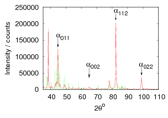
The tempering response of alloy B is shown in figure 6.5. Figure 6.6 shows a plot of the normalised hardness of a variety of steels versus a tempering parameter, defined as T(20 + log t), where T is temperature in Kelvin and t is the time in hours. The normalised hardness is given by (H − Hmin)∕(Hmax − Hmin) where H, Hmax and Hmin represent the hardness, untempered hardness and fully softened hardness as shown in table 6.2. The reason for presenting the data in this way is to allow comparison of the tempering resistance of the bainitic steel against that of a high silicon, quenched and tempered martensitic steel Fe-0.5C-1.3Si wt% [23] and a high silicon, secondary hardening steel Fe-0.34C-5.08Cr-1.43Mo-0.92V-0.4Mn-1.07Si wt% [199]. It is apparent from figure 6.6 that the bainitic steel has a very high resistance to tempering, much higher than the martensitic alloy, and comparable to the secondary hardening steel. The reason is that the precipitation of carbides prevents coarsening of the microstructure as reported for alloy B by Garcia-Mateo et al. [2]. Therefore tempering below ≈550∘C leads to small changes in the thickness of the bainite plates. In alloy B the bainite plates are ≈35 nm before tempering. Changing to 45±4 and 49±4 nm following tempering at 450 and 550∘C for 30 min [2].
Alloy | Hmax | Hmin |
Bainitic steel | 619 | 206 |
Martensitic steel | 820 | 245 |
Secondary hardening steel | 510 | 248 |
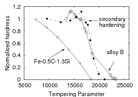
The carbon in the ferrite decreases with tempering temperature and time as shown in figures 6.7 and 6.8. Comparing figures 6.5 and 6.1, it is clear that the hardness cannot be explained by changes in the carbon that is in solid solution alone, the hardness actually increases when alloy B is tempered for 1 h or 30 min at 450∘C while carbon is reducing.
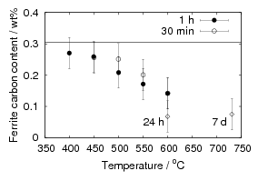
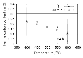
It has been suggested that the excess carbon observed in the bainitic ferrite is located at defects within the ferrite lattice [101, 50, 51]. Plotting the carbon concentration as a function of the measured non–uniform strain (figure 6.9) shows a strong correlation, confirming that the carbon is likely to be located at defects. This might also explain why it does not precipitate easily until the non–uniform strains are relieved by annealing [2].
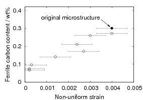
It has long been known that carbon which is segregated to dislocations is stabilised against precipitation, because the segregation itself leads to a reduction in free energy [192].
Tempering for 30 min and 1 h at 400∘C does not introduce any perceptible change compared to the original microstructure of alloy A, when observed using transmission electron microscope, see figures 6.10 and 6.11. This is consistent with the small change in hardness and X–ray analysis of both alloys A and B.
Tempering at 450∘C for 1 h results in the precipitation of carbides which can be observed in transmission electron microscopy, figures 6.12–6.13. Although large austenite regions still seem to be present, carbide precipitation has occurred mainly along the available interfaces between bainitic ferrite plates. Similar observation for the start of carbide precipitation was made on alloy B tempered at 450∘C [2]. There was little difference observed using optical microscopy after tempering, even after 1 h at 600∘C, in that bainite sheaves were still visible, figure 6.14. The main difference being the faster etching in the tempered condition.
As the steel is tempered at progressively higher temperatures the bainite and austenite microstructure decomposes to one of ferrite and carbides (Figures 6.15–6.17). X–ray diffraction of material tempered at 600∘C and carbide extract from the same (figures 6.2 and 6.3), showed that these carbides were predominantly cementite. Thermodynamic calculation indicates that in alloy B cementite is the predominant carbide at equilibrium, with a small increase in amount of M7C3 at lower temperatures. M7C3 becomes stable below around 575∘C in alloy B, and 675∘C in alloy A. At 400∘C in alloy A, M 7C3 is expected in a greater amount than cementite, indicating further changes may take place after prolonged holding at temperature.
As shown in figure 6.18, the hardness seems to decrease towards an asymptotic value during isothermal tempering. As it would be reasonable to expect, at higher temperatures the hardness decrease is greater; after 1 h at 600∘C it falls to around 480 HV, whereas at 700∘C the hardness decreases to 350 HV, similar to that of the pearlite in the same steel.
There is some deviation from general behaviour described above, the hardness after 30 min of tempering often being the same or slightly higher than after 15 min when tempering alloy A. In alloy B which is similar in composition but with higher carbon content the hardness was even observed to substantially increase with particular heat treatments, as a result of precipitating carbides, which are initially fine and well–distributed and therefore contribute strength with greater magnitude than the dissolved carbon lost from the ferrite and austenite.
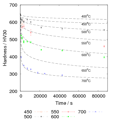
The general change in hardness can be modelled on the basis of Avrami–type kinetic equations (equation 6.1 and 6.2). Hardness values of 650 HV and 250 HV were used for Hmax and Hmin, the initial hardness being used for the maximum, and making an estimate of the minimum hardness encompassing all the results.
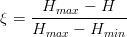 | (6.1) |
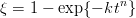 | (6.2) |
where k is a rate constant and n is the Avrami exponent.
Figure 6.19 shows the linear relationships between ln(− ln(1 − ξ)) and ln(t). Linear regression was used to fit the data, listed in table 6.3. As can be seen from the regression coefficient the linear fit is better at higher temperatures. The temptation to infer the mechanisms of transformation was resisted as these may be misleading, but it may be important to note that the gradient of ln(− ln(1 − ξ)) and ln(t) is different for each tempering temperature, indicating that the results may not be explained by a single transformation. A simple model was produced based on Avrami–type equation allowing for linear change of k and n, as shown in table 6.4.
The changes modelled during tempering are the precipitation and growth of cementite particles by partitioning of carbon from the ferrite. At higher temperatures the size of the cementite probably ceases to have a major influence on the strength, because the mean–distance between the particles is the important parameter for strength. The major strengthening mechanism is by the pinning of the nanostructure due to the bainite plate size. Cementite coarsening may have a large influence upon the ability of the ferrite plate size to coarsen. It is unlikely that the various strengthening mechanisms have a linear relationship to particle growth, however it is possible to use an Avrami–type equation as demonstrated by the fitting, as shown in figure 6.18 and comparison of the predictions against actual hardness values in figure 6.20.
| T∕∘C | Intercept C | Gradient m / (ln S)−1 | r.m.s. of residuals |
| 500 | -4.27±0.40 | 0.260±0.045 | 0.20 |
| 600 | -2.29±0.16 | 0.195±0.018 | 0.08 |
| 700 | -1.39±0.21 | 0.207±0.008 | 0.03 |
| Parameter | Intercept | Gradient / (ln S)−1 K−1 | r.m.s. of residuals |
| CT | -0.00026±0.00026 | 0.378±0.14 | 0.031 |
| mT | 0.0144±0.0031 | -11.3±1.9 | 0.44 |
The change in hardness during tempering is more likely to be related to ultimate tensile strength rather then the yield strength. Neither relation is straight–forward so it is better to directly observe changes in each mechanical property. Figure 6.21 shows changes in tensile properties resulting from tempering alloy A. Prior to tempering the ultimate tensile strength was 1.4 GPa with elongation below 1%.
The mechanical properties in these samples were not greatly changed until tempering at 600∘C, whence it was possible to achieve an elongation of 7%, presumably as a result of the decrease in the strain hardening which occurred after 1.2 GPa. Samples tempered at 500∘C also showed increased elongation compared to the base condition and those tempered at 400∘C. Although the failure stress is high, usually above 1.2 GPa, this is does not match the strength achieved in alloy C and D despite the similar microstructure and hardness levels [4, 96]. In those alloys the best combinations of mechanical properties were achieved at transformation temperatures around 250–300∘C, where greater toughness and elongation is displayed. Unfortunately in trying to achieve higher strength by lower transformation temperature the susceptibility to any defects or inclusions is increased due to the smaller critical flaw size (both yield strength increases and toughness decreases as seen in Chapter 1).
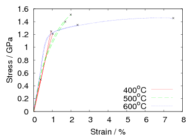
Consistent with previous results discussed in Chapter 1 [3, 101], it has been demonstrated that much of the strength of the virgin microstructure comes from the fine size of the bainite plates in low–temperature bainitic steels. It has been observed that the microstructure is resistant to tempering, and that this is due to the precipitation of carbides as austenite decomposes. It is then difficult for the ferrite plates to coarsen, since the carbides are ideally situated to prevent the movement of ferrite grain boundaries and to contribute to the strength.
In alloy B there is an increase in strength in the early stages of tempering. The strengthening by the precipitation of fine and distributed carbides means that the decomposition of austenite does not lead to any overall softening.
Hardness does not reduce greatly until grain growth starts to occur and is not chiefly dependent upon carbon in solid solution. The carbon concentration in the ferrite slowly decreases as the tempering temperature is increased, concurrent with the recovery of heterogeneous strains. This may help to explain the large supersaturation of carbon in the bainitic ferrite, as being correlated to the high strains in the microstructure caused by the displacive transformation.
Extracted carbides were identified predominantly to be cementite, which is consistent with the rod–like shapes observed using transmission electron microscopy. Calculations using thermodynamic software indicate that M7C3 and vanadium carbides are also to be expected under equilibrium conditions.
The results indicate that bulk austenite may become enriched with carbon after tempering at 400∘C for 30 min and 1 h, but reduced in carbon after tempering at 450∘C.
In chapter 5, the microstructure formed by the bainite transformation at 200∘C was characterised using an atom probe. In this chapter, the same technique is used to examine the changes at nanometre scale during tempering at 400 and 500∘C.
Bainite transformation at low temperature to a material free of carbides results in a novel structure, the tempering behaviour of which has not been characterised extensively. In similarity to virgin martensite there is a supersaturation of carbon in ferrite (1.1±0.7 at.%, ≈0.25 wt%). However, in carbide–free bainite, the austenite is retained in greater amounts and with enrichment in carbon up to the T0 limit (8±1.6 at.%, ≈2 wt% as measured by atom probe in Chapter 5).
Tempering is commonly applied to martensitic steels, to reduce the hardness so as to achieve desirable combinations of strength and toughness. As the metastable microstructure is heated at temperatures where austenite cannot form, several stages of tempering are identified;
First stage: 50–250∘C
Second stage: 200–300∘C
Third stage: 200–350∘C
Fourth stage: above 350∘C
The addition of alloying elements in martensitic steels is generally made to enhance hardenability. Alloying also can accelerate or retard carbide precipitation, and change the temperature ranges of the three stages. Silicon appears to stabilise 𝜖-carbide and retard cementite precipitation, even after tempering at 400∘C [200].
Partitioning during cementite precipitation from supersaturated martensite has been studied using an atom probe by Thompson and Miller [201] in Fe-(0.15,0.4)C-2.25Cr-1Mo wt% steels. Chromium, manganese or molybdenum did not partition after 40 h at 350∘C, consistent with a paraequilibrium, displacive transformation to cementite. After 187 h at 450∘C all three solutes were enriched in the cementite, with greater enrichment in the outer regions of cementite, which were in contact with the ferrite interfaces. Chromium was observed to partition more quickly than manganese or molybdenum. Silicon had partitioned from cementite into the matrix. It was concluded that the diffusion of solutes in the matrix was the rate limiting step in the early stages of enrichment.
Redistribution of carbon in the early stages of tempering has been studied by Miller et al. [202, 203, 204] for iron–carbon and iron–nickel–carbon alloys. It was observed that carbon segregates to lattice defects such as coherent twin boundaries, lath boundaries and high–angle grain boundaries.
The tempering resistance effect due to silicon in martensitic steels was first reported by Owen [8]. Its role in improving resistance to tempering of steels has been studied using an atom probe by Barnard et al. [205] and Chang and Smith [206]. These atom probe studies showed the rejection of silicon from the growing cementite plates. The low solubility of silicon in cementite means that the growth of the plates was inhibited. Therefore later stage kinetics were reported to be controlled by diffusion of silicon rather than carbon. The main influence of silicon was therefore on the third stage tempering rather than on the first. However the major effect of silicon may well be on nucleation of new cementite plates; Ghosh and Olson [207], Lord and Bhadeshia [208] and Kozeschnik and Bhadeshia [209] have shown that nucleation is dramatically reduced or prevented since the potential cementite particle would be forced to accept silicon at the paraequilibrium level.
Atom probe studies were performed using both the energy-compensated optical position-sensitive atom probe (ECO–PoSAP) and the local electrode atom probe (LEAP) method. Tip specimens for atom probe were prepared from 3 mm rods of alloy A, previously transformed into the bainitic condition at 200∘C and tempered for 30 min at 400 and 500∘C.
PoSAP and LEAP experiments were performed with a specimen temperature of 60 K, and pulse fraction of 0.2 of the standing voltage. Pulse repetition rate was 1.5 kHz in PoSAP and 200 kHz in LEAP. The average evaporation rate in LEAP was 2%.
Sample preparation and details of PoSAP have been described in Chapter 5; in this chapter, a local electrode atom probe was also used giving the benefit of a wider field of view, and faster acquisition of data. The combined effect is that some 108 atoms can be acquired, improving the statistical significance of the results.
In the conventional atom probe a 5–10 mm diameter aperture is placed 4–10 mm in front of the specimen tip. In the local electrode atom probe a 20–50 μm diameter aperture is typically positioned 20–50 μm from the specimen. Nishikawa and Kimoto originally proposed such a design for the study of naturally occurring protrusions or ‘micro–tips’ which have a radius of curvature much larger than conventional specimens, as a means of achieving the necessary field strength without having to prepare the traditional needle–shaped specimen [190]. However, when the local electrode is used with a needle shaped specimen it allows the necessary field strengths for field evaporation to be achieved at much lower voltages. This allows usage of voltage pulsers which operate at higher repetition rates, up to 2 MHz, resulting in faster acquisition of data.
The small distance between the local electrode and the specimen improves the mass resolution, meaning that energy compensating lenses are not necessary. This increases the field of view of the specimen that can be analysed. During data reconstruction extra corrections need to be made due to the large field of view, to account for the curvature of the tip.
Alloy A transformed at 200∘C was tempered at 400∘C for 30 min; two composition profiles through the same volume are shown in figures 7.1 and 7.2. The appearance is similar to that previously observed in the as–transformed material. The carbon variation can be attributed to carbon–rich austenite (around 6.5 at.%) and relatively carbon poor ferrite (around 1 at.%), similar to the structure before tempering but with lower carbon contents. Carbon was seen to vary between 0.5–1.5 at.% with an average of 1.01±0.03 at.% (0.25 wt%). Substitutional solutes did not partition between the phases as can be deduced from the profiles. In the small volume observed using PoSAP there was no indication of any carbides except decrease of carbon contents in both the austenite and ferrite. The ferrite and austenite carbon contents are consistent with the X–ray diffraction results.
Caballero et al. [210] have compared the carbon contents of as–transformed low–temperature bainite to that in the tempered condition, in alloy B, to investigate the possibility of the further partitioning of carbon from the ferrite to austenite as exploited in the ‘quenching and partitioning’ process [97]. Caballero et al. concluded that there was no further partitioning of carbon to the austenite during tempering at 400∘C; the carbon content being more strongly affected by the austenite film thickness. However, it is not clear why the carbon would remain in the thin–films, and their results could be interpreted as evidence of partitioning of carbon from thin–films to the remaining blocky austenite, since after tempering the thinner austenite have reduced carbon content and thicker austenite films have higher carbon content compared to films of similar thickness just after transformation.
The austenite observed in this work after tempering at 400∘C may indicate that carbon decreases in austenite during tempering. This could either be a general decrease in all the austenite, or only applicable to thin film austenite; many more measurements would be needed to make the sampling statistically significant due to the large variation in carbon contents in the austenite previously observed in the as transformed steel. Direct measurement of carbon content by atom probe may be particularly useful to characterise the carbon distribution since conventional X–ray diffraction is not able to distinguish the lattice parameters of thin film and blocky austenite after transformation [?].
Calculation with mtdata for this alloy suggests that cementite and M7C3 carbides are stable at equilibrium at tempering temperatures, table 7.1. In this case the carbon content of ferrite is near zero, and austenite is not present. It can also be useful to consider equilibrium between BCC ferrite and FCC austenite. In this condition the austenite volume fraction is expected to decrease and be replaced by ferrite and face–centred–cubic carbides. It was not possible using mtdata to calculate the ferrite–austenite equilibrium, since even when omitting the stronger carbide forming elements vanadium and molybdenum, calculation would predict ferrite and FCC carbides. Paraequilibrium calculations, summarised in tables 7.2 and 7.3, suggest that the carbon in austenite is still below the level expected from paraequilibrium between austenite and ferrite during tempering at 400∘C. This indicates that it would be possible for further carbon to partition to the austenite and even for the amount of austenite to increase if paraequilibrium conditions prevailed. However the paraequilibria between austenite and cementite, or ferrite and cementite, may be more relevant to cementite precipitation; unfortunately this is difficult to calculate because of the lack of experimental data dealing with activity of silicon in cementite.
| Temperature | Phase | mole% | Fe | C | Mn | Si | Cr | Mo | V /at.% |
400∘C | Ferrite | 87.6 | 96 | 0.0 | 0.0 | 3.0 | 0.0 | 0.0 | 0.0 |
| Cementite | 5.3 | 61 | 25 | 10 | 0.0 | 4.0 | 0.0 | 0.0 | |
| M7C3 | 6.7 | 33 | 30 | 19 | 0.0 | 17 | 2.0 | 0.0 | |
| VC | 0.4 | 0.0 | 49 | 0.0 | 0.0 | 0.0 | 18 | 32 | |
400∘C | Ferrite | 92.4 | 97 | 0.0 | 0.0 | 3.0 | 0.0 | 0.0 | 0.0 |
| MC(FCC) | 4.2 | 19 | 48 | 2.0 | 0.0 | 30 | 0.0 | 1.0 | |
| MC(FCC) | 3.4 | 1.0 | 45 | 41 | 0.0 | 8.0 | 4.0 | 2.0 | |
500∘C | Ferrite | 87.2 | 96 | 0.0 | 0.0 | 3.0 | 0.0 | 0.0 | 0.0 |
| Cementite | 7.7 | 59 | 25 | 10 | 0.0 | 6.0 | 0.0 | 0.0 | |
| M7C3 | 4.7 | 34 | 30 | 16 | 0.0 | 18 | 2.0 | 0.0 | |
| VC | 0.3 | 0.0 | 49 | 0.0 | 0.0 | 0.0 | 17 | 33 | |
| T / ∘C | Phase | mole% | Fe | C | Mn | Si | Cr | V | Mo /at.% |
200 | α | 83 | 93.60 | 0.02 | 1.85 | 2.96 | 1.34 | 0.10 | 0.13 |
| γ | 17 | 72.22 | 20.60 | 2.08 | 3.33 | 1.51 | 0.12 | 0.15 | |
300 | α | 80 | 93.55 | 0.05 | 1.85 | 2.97 | 1.34 | 0.10 | 0.13 |
| γ | 20 | 75.50 | 17.51 | 2.02 | 3.24 | 1.47 | 0.11 | 0.14 | |
400 | α | 75.6 | 93.50 | 0.09 | 1.86 | 2.97 | 1.34 | 0.10 | 0.13 |
| γ | 24.4 | 79.02 | 14.13 | 1.99 | 3.18 | 1.44 | 0.11 | 0.14 | |
500 | α | 67.2 | 93.48 | 0.11 | 1.85 | 2.97 | 1.34 | 0.10 | 0.13 |
| γ | 32.8 | 82.77 | 10.48 | 1.96 | 3.14 | 1.42 | 0.11 | 0.14 | |
600 | α | 48.5 | 93.48 | 0.11 | 1.85 | 2.97 | 1.34 | 0.10 | 0.13 |
| γ | 51.5 | 86.66 | 6.72 | 1.92 | 3.08 | 1.39 | 0.11 | 0.14 | |
| Temperature /∘C | Austenite / mole% | Carbon in austenite /at.% |
| 200 | 17.0 | 20.6 |
| 300 | 20.0 | 17.5 |
| 400 | 24.4 | 14.1 |
| 500 | 32.8 | 10.5 |
| 600 | 51.5 | 6.7 |
A second sample tempered at 400∘C was analysed using LEAP. The carbon distribution is shown in figures 7.3(a) and (b). In this volume, a carbide particle was observed with a carbon content around 25±2 at.% with maximum at 28±3 at.%. Figure 7.4(a) shows the carbon atom map for the bainitic steel after tempering at 400∘C for 30 min, with a volume corresponding to 50 nm × 48 nm × 15.5 nm, containing 935 thousand ions. Figure 7.4(b) shows the composition profile. The volume intersects one carbide particle at the edge of the volume, identified by the high carbon concentration. The high carbon content was accompanied by increased nickel and manganese and lower silicon content. The core area of this carbide has almost negligible silicon content and the highest carbon content. An interface of around 2 nm width exists where each element concentration returns approximately linearly to the matrix content. 25 at.% C is equivalent to an M/C ratio 3.0, making this particle most likely to be Fe3C cementite. The ferrite composition in this second volume averages 0.85±0.1 at.% similar to that observed using PoSAP.
Figure 7.5 shows projections of the tomographic element distributions. All elements except silicon appear to segregate to the carbide particles. Similar results can be seen in figure 7.6 after tempering of 500∘C for 30 min.
Figure 7.7 contains carbon atom maps for a sample tempered at 500∘C for 30 min, showing the location of the concentration profiles shown in figures 7.8 and 7.9. The volume studied is 54 nm × 56 nm × 53 nm and contains 3.57 million ions. Features with higher carbon have been labelled from A–E in the order they appear in the profiles, and marked on figure 7.7. Two carbide particles have been identified at C and E, both most likely to be cementite. C has a cylinder shape consistent with cementite formed during tempering, E appears to be more spherical but has been truncated by the edge of the sampling volume. Other features cannot be unambiguously identified.
At A there is depletion of silicon and increased chromium and manganese, trends also observed at C, however carbon is in range 3–4 at.%. At point B carbon and chromium are raised, but other elements are similar to the bulk matrix composition. It is that possible these regions are clusters of carbon, or carbide particles too small to be resolved using the sample volume technique. Previously presented X–ray diffraction results indicate that austenite is not present in this condition.
At D the measured carbon enrichment is up to 10 at.% and the M/C ratio is around 9. At E the carbon is around 20 at.% and the M/C ratio is 4, but the carbon reaches as high as 25 at.% in the centre. In contrast to the carbide at C there is only a slight or no decrease in silicon at D and E. Along with higher carbon, chromium, manganese and nickel as seen at other locations, at D molybdenum is also higher than the surrounding matrix. The main feature transected at D has a rod like shape, around 5 nm across and 20 nm in length, and it possibly has a lower carbon ‘tail’ examining the carbon atom map. The shape is similar to features identified as carbon trapping at dislocations in alloy B (Fe-0.98C-1.46Si-1.89Mn-1.33Cr-0.26Mo-0.09V wt%) after transformation at 200∘C by Caballero et al. [211].
At C the silicon content drops to zero only in the core profile, where the carbon and other elements are highest; apart from this low–silicon core the composition profile is similar to that at D. In previous studies Babu et al. [212] and Thompson and Miller [213] have both observed by atom probe that cementite formed without any initial partitioning of silicon during precipitation from supersaturated martensite in Fe-0.15C-2Si-3Mn wt% and Fe-(0.15,0.4)C-2.2Cr-1Mo-0.3Si-0.5Mn wt%, with silicon only being rejected after prolonged annealing. Bhadeshia and Edmonds [214] after Kalish and Cohen [192] also showed that 𝜖–carbide is not always a precursor to precipitation of cementite in bainitic steels. It therefore seems the whole particle is cementite and that silicon rejection occurs from the centre outwards.
The average carbon content of the ferrite in this region was measured as 1.36±0.1 at.%, with maximum around 2.5 at.% across profile 1 of figure 7.7, and 1.20±0.1 at.% with maximum around 3 at.% across profile 2. The ferrite carbon content was therefore anomalously high compared to the value of 0.85±0.1 at.% observed after tempering at 400∘C.
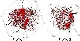
Low temperature bainite formed by transformation at 200∘C of alloy A and subsequently tempered for 30 min at 400 and 500∘C, has been studied using atom probe tomography.
Carbon in ferrite decreased to 1 and then 0.8 at.% respectively after tempering for 30 min at 400∘C and 500∘C. Thin film austenite was observed after tempering at 400∘C. The austenite had lower carbon content (≈6 at.%) than that observed before tempering (≈8 at.%), but many more observations would be needed to assess the significance. The presence of austenite in this condition is confirmed by the earlier X–ray diffraction but the carbon content cannot be reliably measured by X–ray due to the small volume fraction. It is expected that carbon will decrease in the austenite as cementite precipitates, but there is also the possibility for partitioning of carbon from thin–film to blocky austenite.
Carbide particles were identified after both tempering temperatures, with a core of low–silicon. The composition of this low–silicon core matches that for cementite, based on the rejection of silicon and on the metal/carbon ratio. The surrounding carbide is not enriched in silicon as observed in the composition profiles. It seems likely that the growth of the particles is limited by the rate at which silicon can be rejected from the core. The mechanism being similar to that proposed by Owen [8] with the rejection of silicon from cementite into the surrounding matrix limiting the rate of growth.
During tempering the carbides observed are enriched in chromium, manganese and nickel, and reject silicon. They are most likely M3C cementite. The tendency for partitioning of solute elements is the same at both temperatures, but the magnitude of composition change is larger at the higher temperature.
The extremely small size of the carbide particles observed after tempering at 400 and 500∘C for 30 min may help to explain the resistance to tempering, as measured by the change in hardness. Until coarsening occurs a fine dispersion of carbides will add an additional strengthening mechanism.
By transformation at unconventionally low temperatures high–carbon high–silicon steels can produce a microstructure composed of highly refined bainitic ferrite plates in a matrix of retained austenite. The small scale of the plates provides the major strengthening mechanism, and so during tempering the strength is maintained until these plates begin to coarsen.
Calculation of the strength of the microstructure due to its constituent parts showed that the plate size, carbon supersaturation and dislocation density all contribute to the high strength. However, the calculated yield strength based on this model is higher than that observed. It may be that the strength values from martensite theory extrapolate poorly to the bainitic microstructure, in particular regression analysis of the effect of carbon and dislocation density is non–trivial because of the strong correlation between the two. Further work should investigate these relations, by developing the theoretical understanding where possible, and also by further experimental work with mechanical testing and structural characterisation. This could be aided by the compilation of a database of mechanical properties for carbide–free bainitic steels, and the design of critical experiments.
Displacive transformation causes surface relief, due to the small scale of the low–temperature bainite plates, high resolution techniques are required for its characterisation. Observations of the apparent shear component were almost all higher than the expected range of 0.22–0.28, with a mean of 0.31, and a maximum of 0.46. A large shear component is consistent with the more slender aspect ratio of the bainite plates. A comparison should be made against crystallographic theory to establish if such a high value is reasonable from shear alone. Contributions from dilational component or lattice–invariant deformation do not contribute to the shear, but there should also be some consideration of how these can also contribute to the surface relief by distorting the free surface. Further experimental evidence should be collected to confirm the measurements. It would be advantageous if information from below the surface can also be collected to give details of what angle the bainite plate makes with the surface, and to unambiguously identify which features are bainite and which are austenite.
Since the refinement of the microstructure is achieved by transformation, it is unique in providing a path to achieve nano–scale structure in bulk specimens. This has been demonstrated by transformation of a 70 mm block of steel without the use of any special cooling equipment. Procedures exist for the design of such steels, using thermodynamic calculations of martensite start temperature, and time–temperature–transformation kinetics of pearlite and bainite. The Scheil additivity hypothesis has been applied for the calculation of continuous–cooling–transformation. It is proposed that this can be used to design suitable combinations of heat treatments with optimised transformation kinetics. The pearlite reaction in the alloy studied was much faster than calculated in the model utilised for transformation kinetics. This was explained by the observation of pro–eutectoid cementite along prior austenite grain boundaries in the pearlitic samples. This may also have consequences for the mechanical properties in the bainitic condition, since it could greatly reduce the toughness. The pro–eutectoid cementite may be related to the faceted appearance of the fracture surface at the initiation point for failure. There is a need for further experimental evidence to establish the existence and role of pro–eutectoid cementite in these steels. Improved models of pearlite and pro–eutectoid cementite transformation kinetics are critical for the design of bainitic alloys, since they need to be avoided to form fully bainitic structures, and alloying to prevent pearlite formation may also delay the bainite transformation leading to longer transformation times.
Isothermal transformation to bainite at 200∘C resulted in a structure of bainitic ferrite platelets and retained austenite in the form of thin films and blocks. The true plate width of the bainitic ferrite was observed to be 39±1 nm. However, the distribution of plate sizes was not fully explained by the stereological correction applied to measure the true plate width. It may be that further corrections are needed to account for the thickness of the thin foil, or that there may be a wide distribution in the width of bainite plates. This also warrants further research, due to the critical relation of plate size and strength.
Analysis of X–ray diffraction patterns revealed a large supersaturation of carbon in both ferrite (0.3 wt%) and austenite (1.2 wt%) after transformation at 200∘C. This was confirmed by direct measurements using atom probe tomography, with carbon content up to 2 wt% measured in thin films of austenite. The inhomogeneity in the distribution of carbon has stimulated interest because of the role of transformation–induced–plasticity, and also the deleterious influence of insufficiently stabilised blocky austenite.
Transformation at 150∘C produced very interesting results, replicated in two different alloys. Firstly, although the volume transformed was similar to that at 200∘C there was no evidence of carbon partitioning into the austenite. Secondly, the plate width resulting from transformation at 150∘C was wider than at the higher temperature, increasing from 39±1 to 63±4 in alloy A and being 51±4 in alloy C. This was accompanied by an increase in the deviation of the plate sizes, but it is not clear if this is due to increased driving force leading to some coalescence of plates, or due to the formation of an amount of martensite in the microstructure. This is the first suggestion that there may be an optimum temperature at which the smallest bainite plate size can be achieved. Further work should aim at understanding how the fine plate size can best be achieved. Experimental evidence should be collected by identifying compositions which can transform around 200∘C, especially if driving force for transformation and strength of austenite can be varied independently. In the alloys studied so far it may be useful to transform and examine plate sizes at different temperatures (e.g. 250, 225, 175∘C), and to compare histograms of the measurements and the average plate widths. Better understanding of the application of stereological corrections to these thin plates in the volume observed in the thin foils would be useful, as the correction used applies strictly to features intersecting an opaque free surface.
As previously observed, the low–temperature bainitic steels are resistant to tempering. Unlike martensitic steels the strengthening mechanism is mainly by the refined plate size. Fine carbides, which were identified to be cementite, precipitate during tempering and are then ideally situated to prevent movement of the grain boundaries. After tempering at 400 and 500∘C for 30 min the particles were measured to be around 10 nm in diameter. The fine dispersion contributes to the hardness. Carbon in the ferrite was observed to reduce slowly upon tempering, and the loss was associated with recovery of strains as measured by the broadness of the X–ray diffraction peaks. The main focus of this research into tempering was to explain how so much of the hardness was retained by the microstructure after tempering at high temperatures. Further work should be carried out to test how resistant the microstructure is to tempering at lower temperatures, and if the carbide precipitation sequence remains the same. It would be interesting to test whether precipitation occurs when the tempering temperature is the same as the transformation temperature, or whether the structure after transformation is stable to further reactions at the same temperature.
The most common carbide forming in bainitic steels is cementite (𝜃–carbide), and in steels containing large concentrations of silicon, transition carbides such as orthorhombic carbides and 𝜖–, χ–, c– and κ–carbides are formed as they are easier to nucleate. Eventually these carbides transform to cementite if tempering continues.
During typical isothermal heat treatments of the type used to generate bainite, the steel is not held at temperature for periods long enough to permit the long range diffusion of substitutional atoms. This means that 𝜖- and η-carbide or cementite can precipitate within bainitic ferrite, and κ-carbide can precipitate from the carbon enriched austenite between the ferrite platelets. Other carbides require long range diffusion and can form during tempering or during prolonged holding at the isothermal transformation temperature. Crystal structures of carbides in bainite or tempered bainite are shown below in table A.1 [19, 215].
Carbide | Crystal System | M/C |
κ | Hexagonal | 1.37 |
| a=6.9, c=4.8 Å |
|
𝜖 | Hexagonal | 2.4-3 |
| a=2.735, c=4.339 Å |
|
χ | Monoclinic | 2.2 or 2.5 |
| a=11.563, b=3.573, c=5.058 Å, β=97.44∘ |
|
c | Triclinic |
|
| a=6.38, b=5.05, c=4.59 Å, α=90.0∘, β=70.1∘, γ=84.7∘ |
|
η | Orthorhombic | 2 |
| a=4.704, b=4.318, c=2.830 Å |
|
Fe3C | Orthorhombic | 3.0 |
| a=4.525, b=5.087, c=6.743 Å |
|
M7C3 | Orthorhombic | 7/3 |
| a=4.526, b=7.010, c=12.142 Å |
|
(Fe,Si)Cx | Orthorhombic |
|
| a=8.8, b=9.0, c=14.4 Å |
|
(Fe,Si)Cx | Orthorhombic |
|
| a=6.5, b=7.7, c=10.4 Å |
|
(Fe,Si,Mn)Cx | Orthorhombic |
|
| a=14.8, b=11.4, c=8.5 Å |
|
M23C6 | Cubic F | 23/6 |
| a=10.624 Å |
|
M6C | Cubic F | 6 |
| a=11.082 Å |
|
[1] M. J. Peet, S. S. Babu, M. K. Miller, and H. K. D. H. Bhadeshia. Three–dimensional atom probe analysis of carbon distribution in low–temperature bainite. Scripta Materialia, 50, 2004.
[2] C. Garcia-Mateo, M. J. Peet, F. G. Caballero, and H. K. D. H. Bhadeshia. Tempering of a hard mixture of bainitic ferrite and austenite. Materials Science and Technology, 20:814–818, 2004.
[3] F. G. Caballero, H. K. D. H. Bhadeshia, K. J. A. Mawella, D. G. Jones, and P. Brown. Very strong low temperature bainite. Materials Science and Technology, 18:279–284, 2002.
[4] C. Garcia-Mateo and F. G. Caballero. Ultra–high–strength bainitic steels. ISIJ, 45(11):1736–1740, 2005.
[5] F. B. Pickering and T. Gladman. Metallurgical developments in carbon steels. In Special Report No. 81, page 10. Iron and Steel Institute, 1963.
[6] H. K. D. H. Bhadeshia and D. V. Edmonds. Bainite in silicon steels: A new composition–property approach, part 1. Metal Science, 17:411–419, 1983.
[7] H. K. D. H. Bhadeshia and D. V. Edmonds. Bainite in silicon steels: A new composition–property approach, part 2. Metal Science, 17:420–425, 1983.
[8] W. S. Owen. The effect of silicon on the kinetics of tempering. Trans. A. S. M., 46:812, 1954.
[9] C. H. Shih, B. L. Averback, and M. Cohen. Some effects of silicon on the mechanical properties of high strength steels. Trans. A. S. M., 48:86–115, 1956.
[10] K. J. Irvine and F. B. Pickering. Low–carbon bainitic steels. J. Iron Steel Inst., 187:292–309, 1957.
[11] K. J. Irvine, F. B. Pickering, W. C. Heselwood, and M. Atkins. The physical metallurgy of low–C low–alloy steels containing boron. Journal of the Iron and Steel Institute, 186:54–67, 1957.
[12] J. B. Austin. Heat capacity of iron. Ind. Eng. Chem., 24:1225–1235, 1932.
[13] C. Zener. Kinetics of the decomposition of austenite. Trans AIME, 167:550–583, 1946.
[14] J. Kepler. Strena sue de nive sexangula (on the six–cornered snowflake). Frankfurt, 1611.
[15] T. C. Hales and S. P. Ferguson. The Kepler conjecture. Discrete and Computational Geometry, 36:21–69, 2006.
[16] R. W. K. Honeycombe and H. K. D. H. Bhadeshia. Steels: microstructure and properties, 2nd edition. Edward Arnold, London, 1995.
[17] J. C. Anderson and K. D. Leaver. Materials science. Thomas Nelson and Sons, London, 1969.
[18] H. K. D. H. Bhadeshia. Bainite in steels. In G. W. Lorimer, editor, Proceedings of an International Conference: Phase Transformations ’87, pages 309–314, 1988.
[19] H. K. D. H. Bhadeshia. Bainite in steels. The Institute of Materials, London, 1992.
[20] A. G. Guy. Reconstructive and displacive phase transformations. Met. Trans., 3:2535–2536, 1972.
[21] H. K. D. H. Bhadeshia. Bainite in steels. The Institute of Materials, London, 2 edition, 2001.
[22] E. S. Davenport and E. C. Bain. Transformation of austenite at constant subcritical temperatures. Trans. Met. Soc. AIME, 90:117–144, 1930.
[23] E. C. Bain. Functions of the alloying elements in steel. American Society for Metals, Metals Park, Ohio, USA, 1939.
[24] A. Hultgren. J. Iron Steel Inst., 114:421–422, 1926.
[25] G. V. Smith and R. F. Mehl. Lattice relationships in decomposition of austenite to pearlite, bainite and martensite. Trans AIMME, 150:211–226, 1942.
[26] J. M. Robertson. The microstructure of rapidly cooled steel. J. Iron Steel Inst, 119:391–424, 1929.
[27] F. Z. Wever. ”on the transformation in the case of the hardening of steel”. Metallkunde, page 270, 1932.
[28] F. Wever and W. Jellinghaus. Transformation kinetics of austenite. II. dilatometry investigations of austenite decomposition. Mitt. Kaiser–Wilhel Inst. Eisenforschung, 14:85, 1932.
[29] A. Portevin and H. Jolivet. Les transformations au refroidissement dans les aciers. Annales de l’Academie des Sciences Techniques á Varsorie, 4:177, 1937.
[30] A. Portevin and P. Chevenard. The transformations during the cooling of steels. P. Compt. Rend., 204:772, 1937.
[31] J. R. Vilella, G. E. Guellich, and E. C. Bain. On naming the aggregate constituents in steel. Trans. ASM, 24:225–261, 1936.
[32] E. C. Bain. Functions of The Alloying Elements in Steel. American Society for Metals, Cleveland, Ohio, 1939.
[33] R. F. Mehl. Mechanism and rate of decomposition from austenite. In Hardenability of alloy steels, pages 1–65. ASM, 1939.
[34] J. M. Oblak and R. F. Hehemann. Structure and growth of widmanstätten ferrite and bainite. In Transformations and hardenability in steels, pages 15–30, Ann Arbor, Michigan, 1967. Climax Molybdenum.
[35] N. P. Allen, L. B. Pfeil, and W. T. Griffiths. Determination of transformation kinetics in alloy steels. In Second Report of the Alloy Steels Research Committee, Special Report No. 24, pages 369–390, London, 1939. Iron and Steel Institute.
[36] E. P. Klier and T. Lyman. The bainite reaction in hypoeutectoid steels. Trans AIMME, Metals Technology, pages 394–422, 1944.
[37] T. Lyman and A. R. Troiano. Influence of carbon content upon the transformations in 3% chromium steel. Trans. ASM, 37:402–448, 1946.
[38] G. V. Kurdjumov. Discussion section of ‘studies upon Widmansätten structure, IV, the iron–carbon alloys’. Trans. AIMME, 105:253–255, 1933.
[39] R. Entin. The elementary reactions in the austenite – pearlite, bainite transformations. In V.F. Zacky and H.I. Aaronson, editors, Decomposition of austenite by diffusional processes, pages 295–211, New York, 1962. Interscience.
[40] K. C. Russel. The role of quenched–in embryos in solid–state nucleation processes. Metall. Trans., 2(1):5–12, 1971.
[41] D. Yu, D. Chen, D. Zheng, Y. He, and F. Shen. Phase transformation unit of bainitic ferrite and its surface relief in low and medium carbon alloy steels. Acta Metallurgica Sinica A, 2:161–167, 1989.
[42] C. Zener. Equilibrium relations in medium–alloy steels. Trans AIME, 167:513–534, 1946.
[43] F. Wever and H. Lange. The transformation kinetics of austenite. I. magnetic investigations of the decomposition of austenite. Mitt. Kaiser–Wilhelm Inst. Eisenforschung, 14:71–83, 1932.
[44] R. le Houllier, G. Bégin, and A. Dubé. A study of the peculiarities of austenite during the bainite transformation. Trans Metall, 2:2645–53, 1971.
[45] H. K. D. H. Bhadeshia and D. V. Edmonds. The mechanism of bainite formation in steels. Acta Metall., 28:1265–73, 1980.
[46] S. B. Singh. Phase transformations from deformed austenite. PhD thesis, University of Cambridge, 1998.
[47] W. Steven and A. J. Haynes. The temperature of formation of martensite and bainite in low alloy steels. J. Iron Steel Inst., 183:349–359, 1956.
[48] H. K. D. H. Bhadeshia. A rationalisation of shear transformations in steels. Acta. Metall., 29:1117–30, 1981.
[49] A. Hultgren. Isothermal transformation of austenite. Trans. Am. Soc. Metals, 39:915–1005, 1947.
[50] H. K. D. H. Bhadeshia and A. R. Waugh. An atom-probe study of bainite. In Proc. of the International Solid-Solid Phase Transformations Conference, pages 993–998. The Metallurgical Society of the A. I. M. E, 1981.
[51] H. K. D. H. Bhadeshia and A. R. Waugh. Bainite: An atom-probe study of the incomplete-reaction phenomenon. Acta Metallurgica, 30:775–784, 1982.
[52] I. Stark, G. D. W. Smith, and H. K. D. H. Bhadeshia. The element redistribution associated with the incomplete-reaction phenomenon in bainitic steels: An atom-probe investigation. In Proceedings of an International Conference: Phase Transformations ’87, pages 211–215. Institute of Metals, 1988.
[53] I. Stark, G. D. W. Smith, and H. K. D. H. Bhadeshia. The distribution of substitutional alloying elements during the bainite transformation. Metallurgical Transactions A, 21A:847–845, 1990.
[54] B. Josefsson and H. O. Andrën. Atom probe field ion microscopy of bainitic transformation in 2,25Cr-1Mo weld metal. Mater. Sci Technology, 7:849, 1991.
[55] M. Takahashi and H. K. D. H. Bhadeshia. Transition from upper to lower bainite. Mat. Sci. Tech., 6:592, 1990.
[56] K. J. Irvine and F. B. Pickering. High carbon bainitic steels. ISI Spec. Rep., 93:110–125, 1965.
[57] D. N. Shackleton and P. M. Kelly. Morphology of bainite. ISI Spec. Rep, 93:126–134, 1965.
[58] F. B. Pickering. The structure and properties of bainite in steels. In Transformation and hardenability in steels, page 109. Climax Molybdenum, 1967.
[59] S. J. Matas and R. F. Hehemann. The structure of bainite in hypoeutectoid steels. Trans. Met. Soc. AIME, 221:179–185, 1961.
[60] G. R. Srinivasan and C. M. Wayman. Isothermal transformations in an fe–7.9Cr–1.1C alloy. Trans. Met. Soc. AIME, 242:79–81, 1968.
[61] Y. Ohmori and R. W. K. Honeycombe. ICSTIS Suppl. Trans. ISIJ, 11:1160–1164, 1971.
[62] T. Ko and S. A. Cottrell. The formation of bainite. J. Iron Steel Inst., 172:307–313, 1952.
[63] H. I. Aaronson and C. Wells. Sympathetic nucleation of ferrite. Trans AIME, Journal of Metals, 236, 1956.
[64] A. B. Greninger and A. R. Troiano. Crystallography of austenite decomposition. Trans AIMME, 140, 1940.
[65] Z. Nishiyama. X–ray investigation of the mechanism of the transformation from face-centred cubic lattice to body-centred cubic. Sci. Rep. Tohoku Imperial University, 23:325, 1934–1935.
[66] G. Wassermann. Arch. Eisenhüttenwes, 6:347–351, 1933.
[67] G. V. Kurdjumov and G. Sachs. Über den mechanismus der stahlhärtung. Zietschrift für Physik A Hadrons and Nuclei, 64:325–343, 1930.
[68] A. T. Davenport. The crystallography of upper bainite, report on project 12051. Technical report, Republic Steel Research, 1974.
[69] A. Crosky, P. G. McDougal, and J. S. Bowles. The crystallography of the precipitation of α rods from β Cu–Zn alloys. Acta Metall., 28:1495–1504, 1980.
[70] E. C. Bain and N. Y. Dunkirk. The nature of martensite. Trans. AIMME, pages 25–46, 1924.
[71] M. S. Wechshler, D. S. Lieberman, and T. A. Reed. On the theory of the formation of martensite. Transactions of AIMME, 197:1503–1515, 1953.
[72] J. B. Bowles and J. K. Mackenzie. The crystallography of martensite transformations I. Acta Metallurgica, 2:129–137, 1954.
[73] J. K. Mackenzie and J. S. Bowles. The crystallography of martensite transformations II. Acta Metallurgica, 2:138–147, 1954.
[74] D. Hull. The characteristics of the martensite transformation. Bull. Inst. Metals, 2:134, 1954.
[75] B. A. Bilby and J. W. Christian. The Mechanism of Phase Transformations in Crystalline Solids. Monograph No.18. Institute of Metals, 1956. 121–171.
[76] J. W. Christian. The origins of surface relief effects in phase transformations. In Decomposition of Austenite by Diffusional Processes, pages 371–386. AIME, Interscience, 1962.
[77] E. Swallow and H. K. D. H. Bhadeshia. High resolution observations of displacements caused by bainitic transformation. Materials Science and Technology, 12:121–125, 1996.
[78] G. R. Srinivasan and C. M. Wayman. Transmission electron microscope study of the bainite transformation in iron–chromium–carbon alloys. Acta Metallurgica, 16:609–620, 1968.
[79] B. P. J. Sandvik and H. P. Nevalainen. Structure–property relationships in commercial low–alloy bainitic–austenitic steel with high strength, ductility and toughness. Metals Tech., 15:213–220, 1981.
[80] J. D. Watson and P. G. McDougall. The crystallography of Widmanstätten ferrite. Acta Metallurgica, 21(7):961–973, 1973.
[81] B. P. J. Sandvik. The bainite reaction in Fe–Si–C alloys: The primary stage. Metallurgical Transations A, 13A:777–787, 1982.
[82] D. P. Dunne and C. M. Wayman. The crystallography of ferrous martensites. Metallurgical Transactions, 202:2327–2341, 1971.
[83] K. J. Irvine and F. B. Pickering. The impact properties of low carbon bainitic steels. J. Iron Steel Inst., 201:518–531, 1958.
[84] E. R. Morgan, T. E. Dancy, and M. Korchynsky. Improved steels through hot–strip mill controlled cooling. Journal of Metals, 17(8):829–831, 1965.
[85] A. J. DeArdo. Accelerated cooling: A physical metallurgy perspective. In G.E. Ruddle and A.F. Crawley, editors, Accelerated Cooling of Rolled Steel, volume 1, pages 3–27. Metallurgical Society of CIM. Materials Engineering Section, Pergamon Press, 1987.
[86] R. F. Miller, W. G. Benz, and W. E. Unverzagz. Creep strength of 17 low-alloy steels at 1000∘F. Proceedings ASTM, 40:771–781, 1940.
[87] V. F. Zackay, E. R. Parker, D. Fahr, and R. Bush. The enhancement of ductility in high–strengh steels. T. Am. Soc. Metal., 60:252–259, 1967.
[88] O. Matsumura, Y. Sakuma, and H. Takechi. Enhancement of elongation by retained austenite in intercritical annealed 0.4C–1.5Si–0.8Mn steel. Trans. ISIJ, 27:570–579, 1987.
[89] O. Matsumura, Y. Sakuma, and H. Takechi. Trip in its kinetic aspects in austempered 0.4C–1.5Si–0.8Mn steel. Scripta Metall. Mater., 21:1301–1306, 1987.
[90] K. P. Imlau and T. Hellwe. New steel solutions for the worldwide car industry. Steel Research International, 78:180–184, 2007.
[91] K. S. Raghavan, A. S. Sastri, and M. J. Marcinkowski. Nature of the work–hardening behavior in hadfield’s manganese steel. Trans. Met. Soc. AIME, 245:1569–1575, 1969.
[92] C. Garcia-Mateo, F. G. Caballero, and H. K. D. H. Bhadeshia. Development of hard bainite. ISIJ International, 43(8):1238–1243, 2003.
[93] H. K. D. H. Bhadeshia. Hard bainite. In J. M. Howe, D. E. Laughlin, J. K. Lee, U. Dahmen, and W. A. Soffa, editors, Solid→Solid Phase Transformations, TME–AIME, Warrendale, USA, volume 1, pages 469–484, 2005.
[94] F. G. Caballero, H. K. D. H. Bhadeshia, K. J. A. Mawella, and D. G. Jones. Design of novel high strength bainitic steels: Part 1. Materials Science and Technology, 17:512–516, 2001.
[95] F. G. Caballero, H. K. D. H. Bhadeshia, K. J. A. Mawella, and D. G. Jones. Design of novel high strength bainitic steels: Part 2. Materials Science and Technology, 17:517–522, 2001.
[96] M. Y. Sherif. Characterisation and Development of Nanostructured, Ultrahigh Strength, and Ductile Bainitic Steels. PhD thesis, University of Cambridge, 2006.
[97] J. G. Speer, D. V. Edmonds, F. C. Rizzo, and D. K. Matlock. Partioning of carbon from supersaturated plates of ferrite, with application to steel processing and fundamentals of the bainite transformation. Current Opinion in Solid State and Materials Science, 8:219–237, 2004.
[98] P. M. Brown and D. P. Baxter. Hyper strength bainitic steels. In Proceedings of Materials Science and Technology 2004, pages 433–438, New Orleans, Sept 26–29 2004.
[99] H. Qvarnström. Technical note: A mathematical formula for transformation between the steel hardness scales of rockwell C and vickers. Journal of Heat Treatment, 7(65–67), 1989.
[100] B. P. J. Sandvik and H. P. Nevalainen. Structure–property relationships in commercial low–alloy bainitic–austenitic steel with high strength, ductility and toughness. Metals Technology, pages 213–220, June 1981.
[101] C. Garcia-Mateo, F. G. Caballero, and H. K. D. H. Bhadeshia. Low temperature bainite. Journal de Physique, 112:17–25, 2003.
[102] C. Garcia-Mateo. Private communication. Unpublished work, 2002.
[103] C. Garcia-Mateo, F. G. Caballero, and H. K. D. H. Bhadeshia. Acceleration of low–temperature bainite. ISIJ International, 43:1821–1825, 2003.
[104] F. G. Caballero and H. K. D. H. Bhadeshia. Very strong bainite. Current Opinion in Solid State and Materials Science, 8:251–257, 2004.
[105] C. Garcia-Mateo and F. G. Caballero. The role of retained austenite on tensile properties of steels with bainitic microstructures. Materials Transactions, 46(8):1839–1846, 2005.
[106] C. Garcia-Mateo, F. G. Caballero, and H. K. D. H. Bhadeshia. Mechanical properties of low temperature bainite. Materials Science Forum, 500–501:495–502, 2005.
[107] C. G. Mateo and H. K. D. H. Bhadeshia. Nucleation theory for high–carbon bainite. Materials Science and Engineering A, 378A:289–292, 2004.
[108] H. K. D. H. Bhadeshia. Thermodynamic analysis of isothermal transformation diagrams. Metal Science, pages 159–165, 1982.
[109] A. Ali and H. K. D. H. Bhadeshia. Aspects of the nucleation of widmanstatten ferrite. Materials Science and Technology, 6:781–784, 1990.
[110] F. G. Caballero C. Garcia-Mateo. Design of carbide–free low–temperature high strength bainitic steels. Int. J. Mat. Res. (formerly Z. Metallkd.), 98(2):137–143, 2007.
[111] M. Sherif, C. Garcia-Mateo, T. Sourmail, and H. K. D. H. Bhadeshia. Stability of retained austenite in trip–assisted steels. Materials Science and Technology, 20:319–322, 2004.
[112] H. K. D. H. Bhadeshia. Properties of fine–grained steels generated by displacive transformation. Materials Science & Engineering A, 481–482:36–39, 2008.
[113] K. Hase, C. Garcia-Mateo, and H. K. D. H. Bhadeshia. Bimodal size–distribution of bainite plates. Materials Science and Engineering A, A438–440:145–148, 2006.
[114] R. Hammond. Shock and Ballistic properties of bainitic steels. PhD thesis, University of Cambridge, 2004.
[115] R. I. Hammond and W. G. Proud. Does the pressure–induced α → 𝜖 phase transition occur for low–alloy steels. Proceedings of the Royal Society of London A, 460:2959–2974, 2004.
[116] L. C. Chang. Bainite Transformation and Novel Bainitic Rail Steels. PhD thesis, University of Cambridge, 1995.
[117] N. A. Chester and H. K. D. H. Bhadeshia. Mathematical modelling of bainite transforamtion kinetics. J. Phys. IV France, 7(Colloq. C5):41–46, 1997.
[118] S. V. Parker. Modelling of phase transformations in hot–rolled steels. PhD thesis, University of Cambridge, 2004.
[119] A. Ali and H. K. D. H. Bhadeshia. Growth rate data on bainite in alloy steels. Materials Science and Technology, 5:398–402, 1989.
[120] H. K. D. H. Bhadeshia. Kinetics of the bainite transformation. In B.C. Muddle, editor, Proc. 6th Int. Conf. Martensitic Transformations, Sydney, Austrailia, volume 56–58, pages 263–274, Zurich, 1990. Trans Tech Publications.
[121] H. K. D. H. Bhadeshia. Bainite: Overall transformation kinetics. Journal de Physique, Colloq. C4, 12:443–448, 1982.
[122] G. I. Rees and H. K. D. H. Bhadeshia. Bainite transformation kinetics part 1 modified model. Materials Science and Technology, 8:985–993, 1992.
[123] H. K. D. H. Bhadeshia. Large chunks of very strong steel. Materials Science and Technology, pages 1293–1302, 2005.
[124] Hong-Seok Yang. Low–carbon, low–temperature bainite. Master’s thesis, Pohang University of Science and Technology, 2008.
[125] E. O. Hall. The deformation and ageing of mild steel: III discussion of results. Proc. Phys. Soc. London, B64:747–753, 1951.
[126] N. J. Petch. The cleavage strength of polycrystals. J. Iron Steel Inst., 174:25, 1953.
[127] A. Cracknell and N. J. Petch. Frictional forces on dislocation arrays at the lower yield point in iron. Acta Metall., page 186, 1955.
[128] F. N. Rhines. Geometry of grain boundaries. Metall Trans, 1:1105, 1970.
[129] J. P. Naylor. The influence of the lath morphology on the yield stress and transition temperature of martensitic–bainitic steels. Metall. Trans., 10A:861, 1979.
[130] J. Daigne, M. Guttmann, and J. P. Naylor. The influence of lath boundaries and carbide distribtion on the yield strength of 0.4% C tempered martensitic steels. Mater. Sci Eng., 56:1–10, 1982.
[131] C. H. Young and H. K. D. H. Bhadeshia. Strength of mixtures of bainite and martensite. Materials Science and Technology, 10:209–214, 1994.
[132] H. K. D. H. Bhadeshia. Bainite in steels, chapter Mechanical Properties, pages 285–342. The Institute of Materials, London, 2 edition, 2001.
[133] Y. Tomita and K. Okabayashi. Improvement in lower temperature mechanical properties of 0.40 pct C–Ni–Cr–Mo ultrahigh strength steel with the second phase lower bainite. Metallurgical Transactions, 14A:485–492, 1983.
[134] Y. Tomita and K. Okabayashi. Heat treatment for improvement in lower temperature mechanical properties of 0.40 pct C–Cr–Mo ultrahigh strength steel. Metallurgical Transactions, 14A:2387–2393, 1983.
[135] Y. Tomita and K. Okabayashi. Mechanical properties of 0.4 pct C–Ni-Cr–Mo high strength steel having a mixed microstructure of martensite and bainite. Metallurgical Transactions, 16A:73–82, 1985.
[136] G. E. Dieter. Mechanical Metallurgy. McGraw Hill, 1988.
[137] Y. Ohmori, H. Ohtani, and T. Kunitake. The bainite in low carbon low alloy high strength steels. Trans ISIJ, 11:250–259, 1971.
[138] S. B. Singh and H. K. D. H. Bhadeshia. Estimation of bainite plate thickness in low–alloy steels. Materials Science and Engineering A, pages 72–79, 1998.
[139] H. K. D. H. Bhadeshia. Developments in martensitic and bainitic steels: role of the shape deformation. Materials Science and Engineering A, 378A:34–39, 2004.
[140] C. E. Lacy and M. Gensamer. The tensile properties of alloyed ferrites. Trans. ASM, pages 88–105, 1944.
[141] F. B. Pickering and T. Gladman. Metallurgical developments in carbon steels no. 81. Iron and Steel Inst. Spec. Rep., page 10, 1963.
[142] G. R. Speich and H. Warlimont. Yield strength and transformation substructure of low–carbon martensite. J. Iron and Steel Inst., 206:385–392, 1968.
[143] P. G. Winchell and M. Cohen. The strength of martensite. Trans. ASM, 55:347–361, 1962.
[144] K. J. Irvine, T. Gladman, and F. B. Pickering. The strength of austenitic stainless steels. J. Iron Steel Inst., 207(7):1017–1028, 1969.
[145] K. Hase, C. Garcia-Mateo, and H. K. D. H. Bhadeshia. Bainite formation influenced by large stress. Materials Science and Technology, 20:1499–1505, 2004.
[146] J. Frenkel. Über die wärmebewgung in festen und flüssigen körpern. Zietschrift für Physik A Hadrons and Nuclei, 35(8–9):652–669, 1926.
[147] J. W. Morris, Z. Guo, R. Krenn, and Y.-H. Kim. The limits of strength and toughness in steel. ISIJ International, 41(6):599–611, 2001.
[148] D. M. Clatterbuck, D. C. Chrzan, and J. W. Morris Jr. The ideal strength of iron in tension and shear. Acta Materialia, 51:2271–2283, 2003.
[149] S. S. Brenner. Tensile strength of whiskers. J. Applied Physics, 27:1484–1491, 1956.
[150] S. S. Brenner. Growth and properties of “whiskers”. Science, 128(3324):569–575, 1958.
[151] Anonymous. Kobelco technology review. Technical Report 8, Kobe Steel Ltd., Japan, 1990.
[152] F. B. Pickering. Physical Metallurgy and the Design of Steels. Applied Science Publishers, London, 1978.
[153] R. W. K. Honeycombe and H. K. D. H. Bhadeshia. Steels: microstructure and properties, 2nd edition, chapter 10, page 205. Edward Arnold, London, 1995.
[154] T. Yokota, C. Garcia-Mateo, and H. K. D. H. Bhadeshia. Formation of nanostructured steels by phase transformation. Scripta Materialia, 51:767, 2004.
[155] L. Karlsson J. H. Pak, H. K. D. H. Bhadeshia and E. Keehan. Coalesced bainite by isothermal transformation of reheated weld metal. Science and Technology of Welding and Joining, 13:593–597, 2008.
[156] H. K. D. H. Bhadeshia. Alternatives to the ferrite–pearlite microstructures. Materials Science Forum, 284–286:39–50, 1998.
[157] P. B. Burgess and N. F. Kennon. Second stage of tempering. Metals Forum, 4:185–190, 1978.
[158] J. H. Hollomon and L. D. Jaffe. Time–temperature relations in tempering steels. Trans. TMS-AIME, pages 223–249, 1962.
[159] J. Gordine and I. Codd. The influence of silicon up to 1.5 wt% on the tempering characteristics of a spring steel. J. Iron Steel Inst., 1969.
[160] G. R. Speich. In Decomposition of Austenite by Diffusional Processes, pages 353–369. AIME, Interscience, 1962.
[161] G. R. Srinivasan and C. M. Wayman. The crystallography of the bainite transformation I. Acta Metallurgica, 16:621–636, 1968.
[162] H. K. D. H. Bhadeshia. The lower bainite transformation and the significance of carbide precipitation. Acta Metallurgica, 28:1103–1113, 1980.
[163] J. W. Christian. The Theory of Phase Transformations in Metals and Alloys, volume Part 1. Permagon, Oxford, 2 edition, 1965.
[164] J. P. Holman. Heat Transfer. McGraw–Hill Companies, 8 edition, 1997.
[165] A. A. Kaya and D. V. Edmonds. Nonclassical decomposition products of austenite in Fe-C-Cr alloys. Metallurgical and Materials Transactions A, 29:2913–2924, 1998.
[166] H. K. D. H. Bhadeshia. Bainite in steels, page 288. The Institute of Materials, London, 1 edition, 1992.
[167] M. U. Cohen. Precision lattice constants from X–ray powder photographs. Rev. Sci. Instrum., 6:68–74, 1935.
[168] B. D. Cullity. Elements of X–ray Diffraction, page 368. Prentice Hall, 3rd edition, 2001.
[169] W. Parrish and A. J. C. Wilson. Precision measurement of lattice parameters of polycrystalline specimens. In J. S. Kasper and K. Lonsdale, editors, International Tables For X–ray Crystallography, volume 2, pages 216–227. Kynoch Press, 1959.
[170] A. J. C. Wilson. Accuracy in methods of lattice parameter measurement. In Special Publication 567, Proceedings of Symposium on Accuracy in Powder Diffraction held at NBS, MD. National Bureau of Standards, June 11–15, 1979.
[171] M. J. Dickson. The significance of texture parameters in phase analysis by X–ray diffraction. Journal of Applied Crystallography, 2:176–180, 1969.
[172] B. D. Cullity. Elements of X–ray Diffraction, pages 105–137. Prentice Hall, 3rd edition, 2001.
[173] M. Marimuthu. Xrdcalc. http://www.msm.cam.ac.uk/phase-trans/map/, 2002.
[174] M. Marimuthu and M. J. Peet. Xrdcalc1.2. http://mathewpeet.org/thesis/programs/, 2009.
[175] H. M. Rietveld. Line profiles of neutron powder–diffraction peaks for structure refinement. Acta Cryst., 22:151–152, 1968.
[176] H. M. Rietveld. A profile refinement method for nuclear and magnetic structures. J. Applied Cryst., 2:65–71, 1969.
[177] D. J. Dyson and B. Holmes. The effect of alloying additions on the lattice parameter of austenite. J. Iron Steel Inst., 208:469, 1970.
[178] M. J. Peet. LP2C. http://mathewpeet.org/thesis/programs/, 2009.
[179] M.-X. Zhang and P. M. Kelly. Determination of carbon content in bainitic ferrite and carbon distribution in austenite by using cbkldp. Materials Characterization, 40:159–168, 1998.
[180] E. W. Müller. Zh. Tekh. Fiz., 17:412, 1936.
[181] R. H. Fowler and L. W. Nordheim. Electron emission in intense electric fields. Proc. Trans. Roy. Soc. Lond. A, 119:173–181, 1928.
[182] J. R. Oppenheimer. On the quantum theory of the capture of electrons. Physical Review, 31:349–356, 1928.
[183] E. W. Müller. Das feldionenmikroskop. Z. Phys, 31:136–142, 1951.
[184] M. K. Miller. Atom Probe Tomography. Kluwer Academic, 2000.
[185] E. W. Müller, J. A. Panitz, and S. B. McLane. The atom–probe field ion microscope. Rev. Sci. Instrum., 39:83, 1968.
[186] J. A. Panitz. Field desorption spectrometer. US Patent No. 3,868,507, 1975.
[187] M. K. Miller. Presented at the 21st Microbeam Analysis Society meeting, Albuqerque, NM, 1986. unpublished.
[188] A. Cerezo, T. J. Godfrey, and G. D. W. Smith. Application of a position-sensitive detector to atom probe microanalysis. Rev. Sci. Instrum., 59:862, 1988.
[189] T. F. Kelly, P. P. Camus, D. J. Larson, L. M. Holzman, and S. S. Bajikur. On the many advantages of local–electrode atom probes. Ultramicroscopy, 62:29, 1996.
[190] O. Nishikawa and M. Kimoto. Toward a scanning atom probe – computer simulation of electric field. Applied Surface Science, 76/77:424, 1994.
[191] M. K. Miller and K. F. Russel. In–situ phase transformation in the field ion microscope. Surface Science, 246:209–303, April 1991.
[192] D. Kalish and M. Cohen. Structural changes and strengthening in the strain tempering martensite. Materials Science and Engineering, 6:156–166, 1970.
[193] J. O. Andersson, T. Helander, L. Hoglund, and B. Sundman. Thermo–calc & dictra, computational tools for materials science. Calphad, 26:273–312, 2002.
[194] Thermotech Fe–Data Thermodynamic Database. Thermotech Ltd / Sente Software Ltd., Surrey Technology Centre, 40 Occam Road, GU2 7YG, UNITED KINGDOM.
[195] J. W. Christian. Strengthening methods in crystals, pages 261–329. Elsevier, Amsterdam, 1971.
[196] G. K. Williamson and W. H. Hall. X–ray line broadening from filed aluminium and wolfram. Acta Metallurgica, 1:23–31, 1953.
[197] National Bureau of Standards (U.S.). Monogr. 25, 21, 72. (JCPDS–ICDD 2000): PDF number 35–0772, 1985.
[198] NPL. MTDATA. Software, National Physical Laboratory, Teddington, U.K., 2006.
[199] G. P. Contractor, E. G. Schempp, and W. A. Morgan. Carbide composition and microstructure during the tempering of a 5% cr–mo–v steel. ASM Trans. Quarterly, 54(2):208–219, 1969.
[200] R. W. K. Honeycombe and H. K. D. H. Bhadeshia. Steels: microstructure and properties, 2nd edition, chapter 9, pages 171–199. Edward Arnold, London, 1995.
[201] R. C. Thompson and M. K. Miller. The partitioning of substitutional solute elements during the tempering of martensite in Cr and Mo containing steels. Applied Surface Science, 1996.
[202] M. K. Miller, P. A. Beaven, G. D. W. Smith, and S. S. Brenner. Carbon distribution during the aging of iron-nickel-carbon martensites. In H. I. Aaronson, editor, Proceedings International Conference of Solid-Solid Phase Transformations, 1981.
[203] M. K. Miller, P. A. Beaven, and G. D. W. Smith. A study of the early stages of tempering of iron-carbon martensites by atom probe field ion microscopy. Metall Trans, 12A, 1981.
[204] M. K. Miller, P. A. Beaven, S. S. Brenner, and G. D. W. Smith. An atom probe study of the aging of iron-nickel-carbon martensite. Metall Trans, 14A:1021, 1983.
[205] S. J. Barnard, G. D. W. Smith, A. J. Garratt-Reed, and J. Vander-Sande. Atom probe studies: 1) the role of silicon in tempering of steel and 2) low temperature chromium diffusivity in bainite. In Advances in the physical metallurgy and applications of steels, page 33, 1982.
[206] L. Chang and G. D. W. Smith. The silicon effect in the tempering of martensite in steels. J. de Physique, 45-c9:397, 1984.
[207] G. Ghosh and G. B. Olson. Precipitation of paraequilibrium cementite: Experiments, and thermodynamic and kinetic modeling. Acta Materialia, 50:2099–2199, 2002.
[208] H. K. D. H. Bhadeshia, M. Lord, and L.-E. Svensson. Silicon–rich bainitic steel welds. In Proceedings of International Conference: Joining and Welding Solutions to Industrial Problems, pages 43–52, Osaka University, 2003. JWRI.
[209] E. Kozeschnik and H. K. D. H. Bhadeshia. Influence of silicon on cementite precipitation in steels. Materials Science and Technology, 24:343–347, 2008.
[210] F. G. Caballero, M. K. Miller, A. J. Clarke, and C. Garcia-Mateo. Examination of carbon partitioning into austenite during tempering of bainite. Scripta Materialia, 63, 2010.
[211] F. G. Caballero, M. K. Miller, S. S. Babu, and C. Garcia-Mateo. Atomic scale observations of bainite transformation in a high carbon high silicon steel. Acta Materialia, 55:381–390, 2007.
[212] S. S. Babu, K. Hono, and T. Sakurai. APFIM study of the partitioning of substitutional elements during tempering of low alloy steel martensite. Metallurgical Transactions, 25A:499–508, 1994.
[213] R. C. Thompson and M. K. Miller. Carbide precipitation in martensite during the early stages of tempering cr- and mo-containing low alloy steels. Acta Materialia, 46:2203–2213, 1998.
[214] H. K. D. H. Bhadeshia and D. V. Edmonds. Tempered martensite embrittlement: Role of retained austenite and cementite. Metals Science, 13:325–334, 1979.
[215] H. L. Yakel. Crystal Structures of stable and metastable iron-containing carbides. International Metals Reviews, 30(1):17–40, 1985.


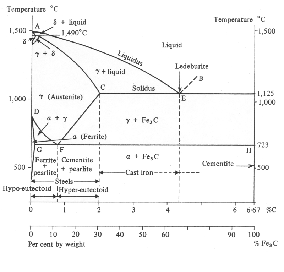
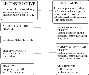
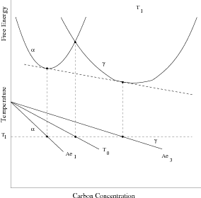
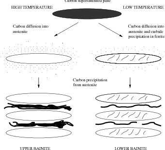

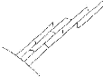

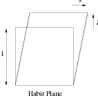

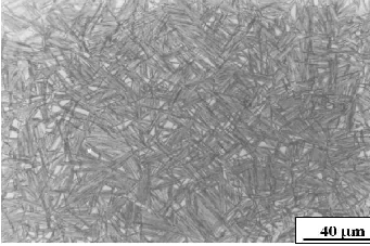
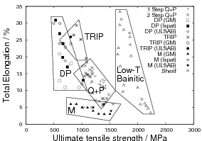
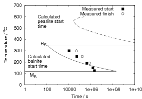

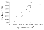
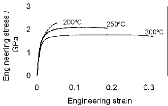
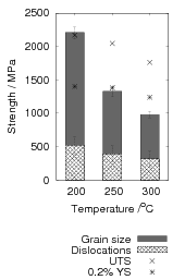
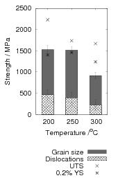
 , 7
, 7